
Ok, first things first: all the R code appearing in all 7/8 of my time-series post is available on GitHub in the repo ‘cool-time-series-stuff
It’s been a while since I last posted on my little time-series journey so I’ll recap:
1. I started with a conceptual problem: I have monthly data on a seasonal process from 

2. In this post I tried to provide some background on important concepts and metrics in time-series analysis. This included a review of important properties of time-series data: stationarity, seasonality, and autocorrelation structure.
3. In a follow-up to #2 I tried to cover autocorrelation in a little more detail, including Breusch-Godfrey tests for serially correlated errors in time-series data.
4. I addressed seasonality here including my understanding of stochastic versus deterministic seasonality.
5. In a 3 part mini-series of posts beginning with this one I tried to introduce Markov Regime Switching processes for seasonal data and describe a popular algorithm (the Hamilton Filter) for estimating Markov Regime Switching Models.
In this post I’m going to talk about (what I see at least) as a philosophical alternative to Markov Regime Switching Models: detecting structural breaks in seasonal data when the number and location of those breaks is unknown.
- Bai (1997) and Bai and Perron (1998) developed statistical tests for detecting the location and number of multiple structural breaks in a time-series.
- Zeileis et al. operationalized this testing procedure and created the R package strucchange for carrying out the operations in R.
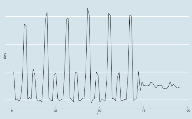
Since it’s been a while since my last time-series post I’m going to start with a fresh empirical set-up. This is a bit manufactured but I work with environmental data all-day, in my off hours I occasionally like to think about other stuff:
Suppose I have data on monthly vacation days taken by people in the San Francisco/San Jose area. From 

Basically we have a process that went from being highly seasonal to one that is almost totally smoothed out.
In my original thinking on this type of problem I was drawn to Markov Regime Switching Models mostly because of the name: I was thinking about this process as consisting of two discrete regimes: a seasonal regime and a smoothed regime…and at some point the process ‘switched’ from one regime to the other. As an empirical matter, I found the results of applying Markov Regime Switching Models to processes like this one pretty unsatisfying…after tinker around with the algorithms employed by software implementing Markov Regime Switching Models (namely R and STATA) one (rather unscientific) conclusion I came to is this: Regime Switching Models like processes that switch back and forth between regimes and they have a comparatively harder time identifying regimes when there is a permanent change.
In theory, since the transition probability between regimes is an estimable parameter, The Hamilton Filter (or any other Markov Regime Switching algorithm) can identify a single one-time break…the implication of such a process is that the maximum likelihood parameter estimate for the transition between regime 2 and regime 1 should approach 0 (once we switch from regime 1 to regime 2, we never switch back to regime 1). In practice, I found that the model had a hard time with processes like the one illustrated above where there was a single change from seasonal to non-seasonal.
To illustrate what I mean by “had a hard time with”, I ran through 10 iterations of a simple replication exercise:
- I simulated data with the same characteristics as the data plotted above
- I used the msm.fit function from the MSwM package in R to fit a Markov Regime Switching Seasonal Regression Model
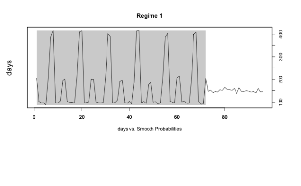
- The package has a built in plotting function plotProb which uses the smoothed probabilities to classify each observation as belonging to either Regime 1 or Regime 2 (it is possible to explore models with more than 2 regimes but I specified a 2 regime model here).
Here is the code for that exercise (in practice I just ran this code block 10 different times):
#first generate some data that has monthly observations on 6 years of a seasonal
#process followed by 2 years of monthly that is not seasonal

year = c(rep(2005,12),rep(2006,12),rep(2007,12),rep(2008,12),rep(2009,12),rep(2010,12))
month = c(rep(1:12,6))

m = c(100,200,300,400)
sig = c(5,10,15,20)
y = c(c(rnorm(1,m[2],sig[2]),rnorm(4,m[1],sig[1]),rnorm(1,m[2],sig[2]),rnorm(2,m[4],sig[4]),rnorm(3,m[1],sig[1]),rnorm(1,m[2],sig[2])),
       c(rnorm(1,m[2],sig[2]),rnorm(4,m[1],sig[1]),rnorm(1,m[2],sig[2]),rnorm(2,m[4],sig[4]),rnorm(3,m[1],sig[1]),rnorm(1,m[2],sig[2])),
       c(rnorm(1,m[2],sig[2]),rnorm(4,m[1],sig[1]),rnorm(1,m[2],sig[2]),rnorm(2,m[4],sig[4]),rnorm(3,m[1],sig[1]),rnorm(1,m[2],sig[2])),
       c(rnorm(1,m[2],sig[2]),rnorm(4,m[1],sig[1]),rnorm(1,m[2],sig[2]),rnorm(2,m[4],sig[4]),rnorm(3,m[1],sig[1]),rnorm(1,m[2],sig[2])),
       c(rnorm(1,m[2],sig[2]),rnorm(4,m[1],sig[1]),rnorm(1,m[2],sig[2]),rnorm(2,m[4],sig[4]),rnorm(3,m[1],sig[1]),rnorm(1,m[2],sig[2])),
       c(rnorm(1,m[2],sig[2]),rnorm(4,m[1],sig[1]),rnorm(1,m[2],sig[2]),rnorm(2,m[4],sig[4]),rnorm(3,m[1],sig[1]),rnorm(1,m[2],sig[2]))
)

df = data.frame(year=year,month=month,days=y)

df2 = data.frame(year=c(rep(2011,12),rep(2012,12)),month=c(rep(1:12,2)),
                  days=rnorm(24,150,7))

z = tbl_df(rbind(df,df2)) %>% mutate(t=seq(1:96))

#plot the series
require(ggthemes)
ggplot(z,aes(x=t,y=days)) + geom_line() +
  theme_economist() + theme(axis.text.y=element_blank())
#-------------------------------------------------------------------

#-------------------------------------------------------------------
require(MSwM)

#Try to identify this break with the MSwM package

#add some monthly dummy variables
z = z %>% mutate(jan=ifelse(month==1,1,0),
                  feb=ifelse(month==2,1,0),
                  mar=ifelse(month==3,1,0),
                  apr=ifelse(month==4,1,0),
                  may=ifelse(month==5,1,0),
                  june=ifelse(month==6,1,0),
                  july=ifelse(month==7,1,0),
                  aug=ifelse(month==8,1,0),
                  sept=ifelse(month==9,1,0),
                  oct=ifelse(month==10,1,0),
                  nov=ifelse(month==11,1,0),
                  dec=ifelse(month==12,1,0))

#look at the simple monthly dummy variable regression
summary(lm(days~factor(month),data=z))

#MRSS with no autoregressive term---------------------------------
mod1 = lm(days~feb+mar+apr+may+june+july+aug+sept+oct+nov+dec,data=z)
mod1.mswm = msmFit(mod1,k=2,p=0,sw=rep(TRUE,13),control=list(parallel=F))
summary(mod1.mswm)
dev.off()
plotProb(mod1.mswm,which=2)
#-------------------------------------------------------------------
Results
| Visually classified | Estimation failure |
| 5 | 3 |
In the table above, visually classified means that the classification of observations in regimes based on the smoothed probabilities looked like this (the area in the shaded gray rectangle is classified as ‘Regime 1’ and the white is classified as ‘Regime 2’):
and the two out of 10 replications that successfully solved for maximum likelihood parameters but that I determined did not correctly classify regimes looked something like this:

Time-series Review
At the risk of being pedantic I think this is good place to pause for a review of the overriding motivations for this foray into time-series:
- I deal with a lot of environmental/economic data and much of the processes I deal with have seasonal components
- I am interested in methods that can help me determine whether a shock (policy changes, environmental changes, etc.) has altered the seasonal pattern of a process
- Because many environmental-economic processes exhibit complex dynamics (regulatory changes happen frequently, biologic/ecologic/hydrologic factors influence processes in frequent, unpredictable ways), I would rather not limit myself to a simple Chow-type test of a structural break at a known point in time.
- I identified two possible paradigms for modeling seasonal processes when the seasonality may be changing: i) smooth transition/regime change models (including state space and random parameters models), and ii) change point detection models (including identification and dating of unknown structural breaks and Bayesian change point models).
- After digging into Markov Regime Switching Seasonal Regressions for a couple weeks, I was left a little unsatisfied regarding their utility in situations where the change in the seasonal process is a true break rather than a switch (in this oversimplified explanation a break means the series never reverts back to the data generating process that was in place before the break…and a switch identifies a process that moves back and forth between a number of known data generating processes).
- That brings us to the present and the current discussion of estimation of number and location of multiple structural breaks
Outline
The remainder of this post is organized as follows:
1. Brief history of testing and dating multiple unknown structural breaks in a data series.
2. Some examples of how to implement the Bai and Perron (2003) approach with the R package strucchange
History
I waffled a little over whether to try and attempt a full formal treatment of this topic….I know math in WordPress can be a little tough on the eyes but, when it comes to models and data analysis, I usually find that I don’t really understand how something works until I can reproduce the math.
Most of you will probably be happy to know that I decided not to go full math-assault on this but rather to just review the key pieces of literature in the development of the topic.
Figuring out how many breaks a time-series has and where they are located evolved from the following seminal contributions:
- The first thing to note is that the well-known Chow test for structural break is inappropriate in the case of an unknown breakpoint. As Hansen (2001) states
An important limitation of the Chow test is that the break date must be known a priori. A researcher has only two choices: to pick an arbitrary candidate break date or pick a break date based on some feature of the data. In the first case, the Chow test may be uninformative, as the true break date can be missed. In the second case the Chow test can be misleading, as the candidate bread date is endogenous – it is correlated with the data – and the test is likely to indicate a break falsely when none exists.
- Going back to 1960 Quandt developed a likelihood ratio test statistic for testing a the hypothesis of a single break when the timing of that break is unknown.
with
The null hypothesis of no structural change is
and the alternative of a single breakpoint at unknown time
is
and
=break fraction
Quandt’s LR statistic for testing
against
when
statistic over a range of break dates
,
= trimming parameters,
.
- Andrews (1993) helped operationalize Quandt’s QLR and the QLR test statistics is often referred to as Andrew’s
statistic.
- Using Andrew’s
- Bai and Perron (2003) outline a dynamic programming procedure for optimally locating a number of structural breaks.


![QLR = max_{m \in [m_{0},m_{1}]} F_{n}(\frac{m}{n})=max_{\lambda \in [\lambda_{0},\lambda_{1}]}F_{n}\lambda](https://s0.wp.com/latex.php?latex=QLR+%3D+max_%7Bm+%5Cin+%5Bm_%7B0%7D%2Cm_%7B1%7D%5D%7D+F_%7Bn%7D%28%5Cfrac%7Bm%7D%7Bn%7D%29%3Dmax_%7B%5Clambda+%5Cin+%5B%5Clambda_%7B0%7D%2C%5Clambda_%7B1%7D%5D%7DF_%7Bn%7D%5Clambda&bg=%23ffffff&fg=%23111111&s=0&c=20201002)
Application
In practice, the R package strucchange will take most of the tedious work out of testing and dating multiple unknown break points in a time-series.
The package allows one to use Andrew’s 
Here is how it work for our data:
require(strucchange)

#first we are going to use the supF test to determine whether the parameters of #our monthly dummy variable regression are stable through the time series:

fs.days = Fstats(days~feb+mar+apr+may+june+july+aug+sept+oct+nov+dec,data=z)
plot(fs.days)

#use the breakpoints functions to find BIC corresponding to optimal number of #breaks
bp.days = breakpoints(days~feb+mar+apr+may+june+july+aug+sept+oct+nov+dec,data=z)

#plot BIC and # of breakpoints...
#the summary() call to the object created by 'breakpoints' returns a list where
# the 'RSS' element of the list is a matrix showing m possible breakpoints and
# the BIC associated with each
bp.plot = data.frame(t(matrix(summary(bp.days)$RSS,nr=2)))
bp.plot$breaks = seq(0:(nrow(bp.plot)-1))

ggplot(bp.plot,aes(x=breaks,y=X2)) + geom_line() + geom_point() + theme_bw() +
  ylab("BIC")
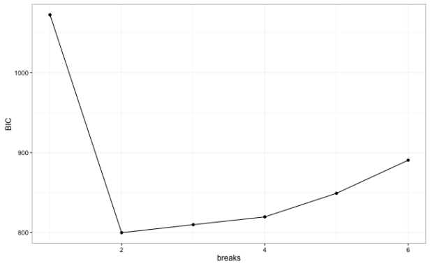
So the method/package appears to correctly identify a single break in our series at 
