
As usual I started with something I thought would be quick, easy, and cool but ended up with something that took longer than it probably should have, morphed into something bigger than I planned, and probably isn’t nearly as cool as it was in my head when I got the idea to do it…but I think it ended up being kind of cool and I can live with that.
I’m going to try and do two things here:
1. present a simple analysis of the return on a set of stock trading recommendations relative to a naive portfolio, and
2. in the context of portfolio management, illustrate a couple potentially interesting uses of R Markdown.
The necessary background is this:
I got a hold of roughly 100 stock trades executed between the fall of 2013 and spring of 2016. The trades are from a subscription service that my dad and I have. The individual we subscribe to makes recommendations that have the following attributes:
- a position (long, short, call, put)
- a trading vehicle (usually a stock or ETF)
- an entry price (buy at $x or lower or short at $y or higher)
- a stop out price (if z closes below $d then get out)
- a target price (this is usually in the form of ‘if it reaches such as such a level start taking profits and if it closes above some other level close out your position’)
A few necessary caveats:
1. I had to throw out several trades because the trading log was hand-written and when I went to put the trades into a spreadsheet I couldn’t tell what some of them were. This is important to recognize because, anecdotally, I’ve observed that some really good traders are wrong way more frequently than they are right. They make a lot of money because they are disciplined about limiting losses when they are wrong and they generally get into trades that have a big upside potential if they are right. Meaning, that taking out even just a few trades could really impact the portfolio performance.
2. I also didn’t include a couple of transactions involving companies that went out of business. I did this because part the routine that I wrote to value the hypothetical portfolio each day includes dynamically loading stock prices from Yahoo Finance…since two of the companies on the trading log are no longer in business, the ticker symbols weren’t valid and Yahoo wouldn’t return historical prices for them. This is important because the trades involving these companies were shorts…i.e. they were probably profitable trades that got left out of the analysis.
I include these caveats to try and focus your attention away from the end result (in this case the trades resulted in a smaller ROI than a naive investment in the S&P would have) and toward the process and the programming output.
Analysis of Trades
Ok, so the trading analysis is pretty simple: in the spreadsheet I recorded each transaction (buy and sell separately) in their own row. An example set of rows for a trade to buy 300 shares of TECS (a leveraged ETF that shorts the technology sector) on 2013-11-13 and sell them on 2013-11-14 would look like:
shares| asset| date | price | option
300 TECS 2013-11-11 24.24 no
-300 TECS 2013-11-14 25.15 no
I know it’s tedious as shit but I haven’t put this stuff in a GitHub repo yet and I don’t have a good way to upload .csv files to a wordpress blog…so if you want the data maybe you can copy and paste the following into your own spreadsheet editor:
date shares asset price option
11/11/13 300 TECS 25.22 no
11/11/13 300 MXWL 7.87 no
11/14/13 -300 TECS 24.74 no
12/13/13 300 MCP 4.58 no
1/6/14 -300 MCP 6.03 no
1/10/14 300 UVXY 15.69 no
1/10/14 150 TECS 21.71 no
1/22/14 -300 UVXY 14.65 no
1/23/14 75 UVXY 60.12 no
1/24/14 -75 UVXY 68.65 no
2/3/14 -150 TECS 23.99 no
2/11/14 50 TSLA 209.15 no
2/18/14 300 TECS 19.94 no
3/5/14 -300 MXWL 15.1 no
3/20/14 -300 TECS 18.8 no
4/4/14 500 TECS 18.45 no
5/22/14 -500 TECS 17.67 no
5/28/14 -100 WDC 87.1 no
5/28/14 100 UVXY 38.5 no
5/29/14 100 WDC 83 no
6/3/14 250 TECS 16.65 no
6/5/14 -100 UVXY 33.73 no
6/5/14 -250 TECS 16.31 no
6/5/14 1000 ZNGA 2.9 no
6/27/14 -1000 ZNGA 3.23 no
7/7/14 -100 GME 41.61 no
7/10/14 100 GME 41.98 no
7/10/14 300 TECS 15.48 no
8/12/14 -300 TECS 14.19 no
8/12/14 1000 ALU 3.23 no
8/12/14 1000 ZNGA 2.82 no
8/14/14 100 GME 47.54 no
8/26/14 -1000 ALU 3.33 no
8/26/14 -1000 ZNGA 2.92 no
9/5/14 -300 GLW 21.07 no
9/18/14 1 SSYS 4.8 yes
9/22/14 200 TECS 13.08 no
10/10/14 -1 SSYS 13.45 yes
10/13/14 300 GLW 18.03 no
10/13/14 700 GTAT 0.52 no
10/14/14 -200 TECS 15.49 no
10/14/14 -700 GTAT 0.41 no
10/22/14 300 TECS 14.28 no
10/24/14 150 SQQQ 36.03 no
10/28/14 -300 TECS 13.24 no
10/28/14 -150 SQQQ 33.87 no
10/29/14 1 TECS 1.1 yes
11/6/14 1000 MCP 1.3 no
11/11/14 500 ZNGA 2.59 no
11/20/14 -1 TECS 0.21 yes
11/20/14 200 DDD 35.87 no
11/21/14 -1000 MCP 1.14 no
11/21/14 -500 ZNGA 2.68 no
12/1/14 -200 DDD 33.42 no
12/10/14 -50 WDC 108.94 no
12/18/14 50 WDC 111.91 no
12/18/14 1 WDC 4.46 yes
12/26/14 1 STX 1.79 yes
1/5/15 150 TECS 11.5 no
1/26/15 -1 STX 7.92 yes
1/26/15 100 SQQQ 28.84 no
2/3/15 -50 TSLA 215.02 no
2/11/15 -100 SQQQ 27.07 no
2/13/15 -150 TECS 10.12 no
2/20/15 500 MXWL 6.48 no
3/19/15 300 MXWL 7.45 no
3/19/15 300 DDD 27.36 no
3/30/15 -300 DDD 27.21 no
4/1/15 -500 MXWL 7.87 no
4/1/15 -300 MXWL 7.87 no
4/17/15 -50 WDC 99.53 no
4/17/15 1 WDC 2.13 yes
5/14/15 50 WDC 97.67 no
5/14/15 -1 WDC 2 yes
5/26/15 100 TECS 36.52 no
5/28/15 -50 WDC 99.42 no
7/6/15 50 WDC 78.89 no
7/13/15 -100 GME 47.27 no
7/20/15 -100 TECS 34.24 no
7/23/15 500 ZBIO 17.75 no
8/5/15 100 TECS 36.71 no
8/5/15 -100 WDC 85.41 no
8/13/15 -300 ZBIO 20.8 no
8/14/15 -200 ZBIO 21.74 no
8/14/15 -100 TECS 37.65 no
8/14/15 100 WDC 82.14 no
8/25/15 500 MXWL 4.66 no
9/10/15 200 DDD 13.1 no
9/29/15 -500 MXWL 5.32 no
9/29/15 -200 DDD 11.02 no
10/8/15 -50 WDC 84.3 no
10/8/15 -50 GME 43.74 no
10/20/15 50 GME 44.78 no
10/22/15 50 WDC 69.52 no
10/22/15 100 TECS 33.65 no
10/22/15 -100 TECS 33.41 no
12/7/15 200 DDD 9.15 no
12/29/15 -200 DDD 9.15 no
12/30/15 100 TECS 29.41 no
12/30/15 25 TSLA 241.38 no
1/11/16 -25 TSLA 206.47 no
3/10/16 200 TECS 31.01 no
5/3/16 -50 DLR 89.01 no
5/5/16 50 TECS 30.3 no
5/16/16 50 DLR 97.52 no
5/16/16 -50 TECS 28.75 no
The basic logic of the routine I wrote is super simple:
1. assume we start with $50,000. I don’t know how much was in the account that these actual trades came from but no single trade was more than $10,000 so $50k seem reasonable.
2. we start the day before the first trade was recorded and establish a data frame of ‘open positions.’ In this case, the trading log had 17 distinct vehicles that were traded over the sample period. I made a data frame for the beginning portfolio that had a row for each vehicle and 0 shares recorded for each row…except the ‘CASH’: there were 50,000 shares of CASH at $1/share
#load packages
library(ggplot2)
library(lubridate)
library(data.table)
library(quantmod)
library(dplyr)
library(zoo)

#read in the data
df.dw = tbl_df(read.csv("techinsiderportfolio.csv"))

#for this first pass there are a couple of things that are problematic:
# 1. two ticker symbols aren't recognized by Yahoo finance because they
# are for companies that don't exist anymore: GTAT & MCP
#2. the options trades weren't recorded with enough information to correctly
#   value them.
# I solve both problems by just removing the problematic trades

df.dw <- df.dw = filter(!asset %in% c('GTAT','MCP')) %>%
                  filter(option=='no') %>%
        mutate(tradedate=as.Date(date,format="%m/%d/%y"),
               asset=as.character(asset)) %>%
        select(shares,asset,price,tradedate,option)

names(df.dw) <- c('shares','asset','price','date','option')

#-------------------------------------------------------
#get prices for each asset in the trading log for every
# day starting with the first trade in the log and
# ending with the last trade

start.date <- min(df.dw$date)
end.date <- max(df.dw$date)

prices <- df.pull(tickers=c('TECS','MXWL','UVXY','TECH',
                            'WDC','ZNGA','GME','ALU','GLW',
                            'SSYS','SQQQ','DDD','STX',
                            'TSLA','ZBIO','DLR'),startDate=start.date,endDate=end.date)
#----------------------------------------------------------

#---------------------------------------------------------
#set up a data frame of positions open on the day before
# the first day...this will only have an open position
# for cash.
open.positions <- data.frame(rbind(data.frame(shares=0,
                                asset=unique(df.dw$asset),costbasis=NA,saleprice=NA),
                                   data.frame(shares=50000,asset='CASH',costbasis=1,saleprice=1)))
open.positions$asset <- as.character(open.positions$asset)

   shares asset costbasis saleprice
1       0  TECS        NA        NA
2       0  MXWL        NA        NA
3       0  UVXY        NA        NA
4       0  TSLA        NA        NA
5       0   WDC        NA        NA
6       0  ZNGA        NA        NA
7       0   GME        NA        NA
8       0   ALU        NA        NA
9       0   GLW        NA        NA
10      0  SQQQ        NA        NA
11      0   DDD        NA        NA
12      0  ZBIO        NA        NA
13      0   DLR        NA        NA
14  50000  CASH         1         1

#set up the skeleton of a portfolio data frame
portfolio <- rbind(data.frame(shares=50000,
                              asset='CASH',
                              date=start.date-1,
                              val=50000,
                              costbasis=1,
                              saleprice=NA,
                              Close=NA),
                   data.frame(shares=0,
                              asset=unique(df.dw$asset),
                              val=0,
                              costbasis=NA,
                              saleprice=NA,
                              date=start.date-1,
                              Close=NA)
                    )
#------------------------------------------------------------
ndays <- length(unique(prices$date))
3. We loop through each day and follow a couple simple steps:
A. we get any new positions (purchases or sales) initiated on that day from the original data frame of trades and we use these new positions to calculate the change in our cash position…if new shares were bought, the value subtracts from the current cash position and if the shares were sold the value is added to the cash position.
B. we append the new positions to current data frame of open positions then we aggregate by asset. this step is creating the ‘net position’ for the current day.
C. we merge the data frame of open positions with the daily prices that were pulled from Yahoo Finance. Here we use the closing price of each open position to value it…so we are basically calculating the value of each open position at the end of the current day.
for(iday in 1:ndays){

    d.now <- unique(prices$date)[iday]
    #get today's prices
    p <- prices %>% filter(date==d.now) %>%
    select(Close,asset,date)

    #first we amend open.positions with the current day
    open.positions <- open.positions %>% mutate(date=d.now) %>%
                      left_join(p,by=c('asset','date'))

    #next we get the new positions and add them to the end of open positions
    change.to.cash <- as.numeric(df.dw %>% filter(date==d.now) %>%
                      mutate(v=shares*price) %>%
                      summarise(v=sum(v)) %>% select(v))

    new.positions <- df.dw %>% filter(date==d.now) %>%
                      mutate(costbasis=ifelse(shares>0,price,NA),
                             saleprice=ifelse(shares<0,price,NA),                              Close=0) %>%
                      select(shares,asset,costbasis,saleprice,date,Close)

    open.positions <-rbind(open.positions,new.positions)

    #adjust cash in the open positions and adjust the net shares of each asset
    open.positions <- open.positions %>%
        mutate(shares=ifelse(asset=='CASH',shares-change.to.cash,shares),
               Close=ifelse(asset=='CASH',1,Close)) %>%
        group_by(asset,date) %>%
        mutate(totalshares=sum(shares),
               w=ifelse(totalshares!=0,shares/totalshares,0),
                cbnew=ifelse(totalshares!=0,w*costbasis,costbasis),
               spnew=ifelse(totalshares!=0,w*saleprice,saleprice)) %>%
       summarise(shares=sum(shares),
                 Close=max(Close),
                 costbasis=sum(cbnew,na.rm=T),
                 saleprice=sum(spnew,na.rm=T)) %>%
        mutate(val=shares*Close)

    portfolio <- rbind(portfolio,open.positions)

#now we clean up the open.positions data frame so it can be updated
open.positions <- open.positions %>% select(shares,asset,date,costbasis,saleprice)
}
Ok, I stand by my assessment that the routine is really simple…but I realize there are a few messy looking dplyr pipings in there that might make it look confusing. Let me comment on those real quick and see if anybody wants to suggest a better way to do things:
- the second to last dplyr chain involving the ‘open.positions’ data frame has kind of a strange routine to take the weighted averages of the cost basis and sale prices. I did this because I wanted to be able to carry around the cost basis so I would be able to calculate the profit or loss from each trade. Sometimes we buy shares of an asset at a certain price then, before we sell those shares, we buy more at a different price. The weighted averaging works to keep the cost basis correct throughout the length of time that a long position stays open.
- I do the same weighted averaging for the sale price. I don’t think it matters in this case because I don’t think there were any instances of shorting a stock, then shorting more at a different price before covering…but if that did happen I think the way I did the selling price aggregation would be the right way.
Ok, so let’s compare the evolution of this portfolio with what $50,000 invested in an S&P index would have done over the same time period:
#pull historical S&P growth over the relevant time period
idx = c('^GSPC')
sp = df.pull(tickers=idx,startDate=start.date,endDate=end.date)

#calculate growth relative to value on day one of the comparison
sp.start = sp$Adjusted[1]
sp = sp %>% mutate(g=Adjusted/sp.start,portfolio='S&P') %>%
      select(date,g,portfolio)
v.start = v$value[1]
v = v %>% mutate(g=value/v.start,portfolio='TI') %>%
      select(date,g,portfolio)

#plot the returns
comp = rbind(v,sp)
ggplot(comp,aes(x=date,y=g,color=portfolio)) + geom_line() + ylab('% gain')+
  xlab('') + scale_color_manual(values=c('black','blue')) + theme_bw()

It’s not great for the expert (the ‘TI’ portfolio on the plot above)…but remember my caveats from earlier: there were some data issues that might be biasing my representation of the return on the expert portfolio.
One substantive comment that might be worth thinking about: the trading portfolio I evaluated here suffers mostly because the majority of the portfolio is sitting in cash most of the time. I guess there are good reasons for experienced traders to have big cash positions most of the time (most of your trades are going to be small potatoes but every once in a while a really profitable situation arises and you want to be ready to go big when the risk-reward ratio is high) but, in this case, that money on the sidelines is incurring a big opportunity cost.
An R Markdown Example
I’ve been wanting to get up to speed on R Markdown for a while…and specifically, the following use-case:
Suppose you have a database that gets updated frequently with something like short-term stock trades. Maybe you’re a fund manager and you want to be able to get daily or weekly reports on portfolio activity. I can think of a few other cases where frequent low-level summaries of ever-changing data would be useful but let’s run with this one for now.
A few good R Markdown tutorials are here:
- http://rmarkdown.rstudio.com/
- https://blog.rstudio.org/2014/08/01/the-r-markdown-cheat-sheet/
- http://rpubs.com/mansun_kuo/24330 – this one has a fair amount of weird Chinese stuff on it but there’s some helpful info peppered in too.
I’m going to use R Markdown to generate a weekly report of trading activity.
I’m going to keep this super simple. The logic of what I’m going to do is this:
- The portfolio I created with the code above has a set of positions (most are 0, some are short positions and some are long positions) for every day.
- Write a function in R that accepts as inputs a value for year and week.
- Given a year and week, the function will return a data frame that has a summary of all positions that changed during that week and year.
- I insert this function into an R Markdown document and, by knitting the R Markdown document, we get a report of the position changes for the given week/year.
- Since the report is created with a function, we can simply change the values for week and year and get a new weekly report.
First, the function to get changes to each position for a given week and year:
#================================================================
#================================================================
#create a function to display all position changes for a particular
# week
changes = portfolio %>% group_by(asset) %>% arrange(asset,date) %>%
          mutate(diff=shares-lag(shares),week=week(date),year=year(date)) %>%
          ungroup() %>% mutate(id=row_number())

#----------------------------------------------------
#write a function which takes the inputs week and year and
# looks for any changes to any position during that week
# the function will then set up data that can be displayed in a table
# with the following structure:

# asset|position|date|new position|date|return

position.sum.wk = function(wk,yr){
#generate a list of asset names for positions that changes this week
tradeids = changes$id[changes$week==wk & changes$year==yr & changes$diff!=0 &
                            changes$asset!='CASH' & is.na(changes$diff)==F]

history.fn = function(tid){
    t.date = changes$date[changes$id==tid]
    a = changes$asset[changes$id==tid]
    hist.df = changes[changes$date<t.date & changes$asset==a,]          #find he latest date in the data frame for which the position was 0     pos0 = max(hist.df$date[hist.df$shares==0])          hist.df = changes %>%
      filter(changes$date>= pos0 & changes$date<=t.date & asset==a)

return(hist.df)
}

lapply(tradeids,history.fn)
}
#----------------------------------------------------
#================================================================
#================================================================
Ok, I don’t want to be too hand-wavy about what this function is doing so let me flush it out a little bit:
Step 1: create a data frame called ‘changes’ that has a column called ‘diff’. The value in this column is the difference between the current position and last position. Example, on 2013-11-14, we sold 300 shares of TECS. On 2013-11-13 the value of ‘shares’ for TECS was 300 and on 2013-11-14 it was 0. Therefore, on 2013-11-14 there is a value of -300 for ‘diff’.
Step 2: For a given week and year find all the entries in the data frame ‘changes’ where diff is not equal to 0…i.e. all the rows representing a change in a particular position.
Step 3: For any particular row where diff is not equal to 0 (any particular transaction), find the latest (most recent) date which is less than the transaction date where the position for that asset was 0…that is, find the start of this particular position.
Step 4: Create a data frame for the current asset which include all the data between the start of the position and the change in the position. For example, we bought TECS on 2013-11-11. We sold TECS on 2013-11-14. For the TECS transaction on 2013-11-14, 2013-11-10 was the most recent date for which our TECS position was 0. We want to create a data frame with all the data on TECS from 2013-11-10 to 2013-11-14. This gives us the complete history of that transaction (the one on 2013-11-14 that closed out the position).
Step 5: do this for all of the other rows where diff is not equal to 0 and save each in it’s own data frame.
Next, we put this function inside an R Markdown document. Let’s back-up and do this step by step:
- In R Studio go File–>New File–>R Markdown. This will open a new R Markdown document
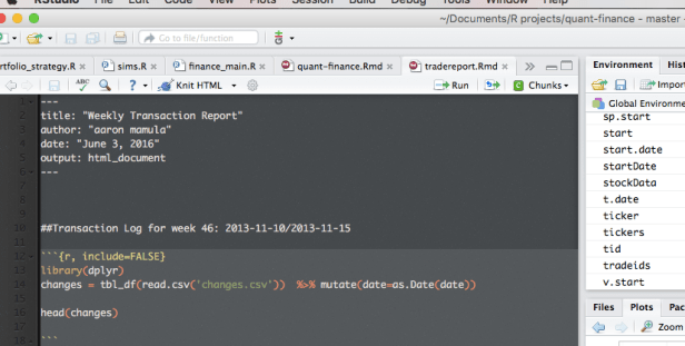
- The new document will have a bunch of boiler plate. Replace the boiler plate with the code below
---
title: "Weekly Transaction Report"
author: "aaron mamula"
date: "June 3, 2016"
output: html_document
---
##Transaction Log for week 46: 2013-11-10/2013-11-15
```{r, include=FALSE}
library(dplyr)
changes = tbl_df(read.csv('changes.csv')) %>% mutate(date=as.Date(date))
head(changes)
```
```{r, echo=FALSE}
position.sum.wk = function(wk,yr){
#generate a list of asset names for positions that changes this week
tradeids <- changes$id[changes$week==wk & changes$year==yr & changes$diff!=0 &
changes$asset!='CASH'& is.na(changes$diff)==F]
history.fn <- function(tid){
t.date <- changes$date[changes$id==tid]
a <- changes$asset[changes$id==tid]
hist.df <- changes[changes$date<t.date & changes$asset==a,]
#find he latest date in the data frame for which the position was 0
pos0 <- max(hist.df$date[hist.df$shares==0])
hist.df <- changes %>%
filter(changes$date>= pos0 & changes$date<=t.date & asset==a) %>%
select(shares,asset,date,costbasis,saleprice,Close,diff)
names(hist.df) = c('open position','asset','date','costbasis','saleprice','Close','diff')
return(hist.df)
}
lapply(tradeids,history.fn)
}
```
```{r,include=FALSE}
dlist=position.sum.wk(wk=46,yr=2013)
```
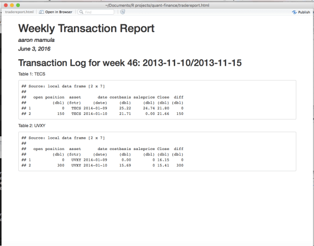
Table 1: `r unique(dlist[[1]]$asset)`
```{r,echo=FALSE}
dlist[[1]]
```
Table 2: `r unique(dlist[[2]]$asset)`
```{r,echo=FALSE}
dlist[[2]]
```
Table 3: `r unique(dlist[[3]]$asset)`
```{r,echo=FALSE}
dlist[[3]]
```
A few things to point out about the R Markdown doc:
- the chunks beginning with “`{r} are code chunks. we put R code here and when we compile the markdown document (knit), it runs the code and includes the output in our document.
- one of the first chunks in my R Markdown above has the familiar library(dplyr) and read.csv() calls. Even though I opened my R Markdown document from an open R Studio project and the dplyr package was previously loaded into the workspace for the project, R Markdown somehow doesn’t know that…so we need to tell it. This is also true of whatever data we want to use – the data are in the workspace but we need to explicitly load them into the markdown doc (I’ll say more about this in a sec).
Final note of procedure: I have an R Markdown doc open in my active R Studio project. I have inserted the code chunks I need in my markdown doc. To compile the doc to an html output file all I need to do is ‘knit’ it. In the image below not there is an icon that says, ‘knit HTML’ in the top banner just below my script tabs:
R Studio ships with the package ‘knitr’ and this icon calls the ‘knitr’ routines that turn the R Markdown doc into a nice HTML doc. When I ‘knit’ the R Markdown with code I pasted above I get the following weekly transaction report:

Final Wrap-Up
1. Let’s go back to that read.csv() call in the R Markdown document. In practice, I could have embedded all the code displayed in this post inside the R Markdown document and made the Weekly Trading Report entirely self-contained. I didn’t want to do that. In order to avoid doing that, I ran most of this code in R then shipped the data frame object ‘changes’ off the a .csv. Then I read that .csv into the R Markdown doc.
In practice, I think the real strength of dynamic document making using R Markdown would be better displayed in the following circumstance:
- imagine we already had a database with all of our trades in it.
- we updates this database with all the activity from the current week.
- then we open our R Markdown document, change the ‘wk’ value in the position.sum.wk() function to the current week, change the ‘yr’ value to the current year, knit the document and voila! We have a new weekly report.
This could be easily accomplished if we just replace the read.csv() call with the appropriate use of RODBC functions and SQL queries to pull the relevant data.
Just to illustrate the potential utility of this, note that the screenshot above has a weekly report for week 46 of year 2013. Let’s pretend we were in week 46 of 2013 last month. Now a few weeks have passed and we want our new weekly report, we just change the two input values to the position.sum.wk() function (here we get a new weekly report for week 2 of 2014):
---
title: "Weekly Transaction Report"
author: "aaron mamula"
date: "June 3, 2016"
output: html_document
---

##Transaction Log for week 2: 2014-01-07/2014-01-12

```{r, include=FALSE}
library(dplyr)
changes = tbl_df(read.csv('changes.csv'))  %>% mutate(date=as.Date(date))

head(changes)

```

```{r, echo=FALSE}

position.sum.wk = function(wk,yr){
#generate a list of asset names for positions that changes this week
tradeids <- changes$id[changes$week==wk & changes$year==yr & changes$diff!=0 &
                         changes$asset!='CASH'& is.na(changes$diff)==F]
history.fn <- function(tid){
 t.date <- changes$date[changes$id==tid]
    a <- changes$asset[changes$id==tid]
    hist.df <- changes[changes$date<t.date & changes$asset==a,]
   #find he latest date in the data frame for which the position was 0
    pos0 <- max(hist.df$date[hist.df$shares==0])
      hist.df <- changes %>%
      filter(changes$date>= pos0 & changes$date<=t.date & asset==a) %>%
        select(shares,asset,date,costbasis,saleprice,Close,diff)
  names(hist.df) = c('open position','asset','date','costbasis','saleprice','Close','diff')
return(hist.df)
}
lapply(tradeids,history.fn)
}

```

```{r,include=FALSE}
dlist=position.sum.wk(wk=2,yr=2014)
```

Table 1: `r unique(dlist[[1]]$asset)`
```{r,echo=FALSE}
dlist[[1]]
```

Table 2: `r unique(dlist[[2]]$asset)`
```{r,echo=FALSE}
dlist[[2]]
```
Then we knit our R Markown doc and get:
2. As with most things I do here, you can do way cooler shit with R Markdown than just a shabby little weekly report that barfs out a few data frames. If one wanted to graphically display the weekly change in portfolio value each week there are endless possibilities for doing just that.
