I started working with R Notebooks pretty recently and I really, really, really, really like them. I haven’t done anything sophisticated with them yet so I’m going to try to keep this post pretty short. He’s what I’m aiming for today:
- Tell you why I think R Notebooks are cool and provide an example of a functioning Notebook.
- Give you some specific instructions on how to start using notebooks (the kind of stuff you could just Google off the interwebs….but I’m trying to be a full-service type of shop here).
Why are R Notebooks Cool?
R Notebooks allow you to combine text, equations, and code to produce a slick looking document. A key difference between R Notebooks and plain old vanilla R Markdown Documents is that R Notebooks allow you to have code chunks that can be run independently and interactively.
A use-case where this functionality really shines in teaching. Think of the way a lot of us learned econometrics. Basically, we worked through Bill Greene’s big book of idempotent matricies then, at some point, we had to do a homework assignment that involved actual data and we shit our pants…then a lot of us without a strong programming background did one of two things:
1. Jacked around in Gauss or C forever trying to figure out how to do 
2. Went straight to some black-box application, did some version of:
reg y x
which did nothing to strengthen our understanding of the OLS estimator.
Notebooks (in this case R Notebooks) make great teaching tools because you can combine:
1. Text – such as a conceptual discussion of what linear regression is about and,
2. Equations/Math – such as a rigorous derivation of the OLS estimator and,
3. Interactive Code that the student can run to deepen their understanding of what the estimator is and how to implement it is a ‘real world’ type situation.
Example
Here is a great example of where the independent code execution feature comes in handy. It was provided by a colleague of mine who taught a short course on time-series analysis using an R Notebook. The notebook covered a range of topics and one code chunk in particular was designed to caution against making judgements regarding stationarity of a time-series based on plots. He set up the following simulation:
library(xts)
library(KFAS)

x = arima.sim(list(order=c(2,0,0),ar=c(1,-0.9),n=2^8)
ts.plot(x)
In water-down terms a stationary time-series should have a mean and variance that don’t change over time….however, using the code above to generate series from a process that is known to be stationary we can see that this process often generates series that LOOK non-stationary.
The cool thing about setting this code chunk up in an R Notebook is that other code chunks in the same notebook can contain modules that do other things like read in big data sets and use them to run models…but since the simulation is it’s own chunk it can be run, re-run, and played with by the user without having to run all the other chunks (some of which might do time-intensive things).
An R Notebook for my Average Treatment Effects Project
In my last post I set out to replicate a variety of average treatment effect estimators discussed in this post on The STATA Blog. My main motivation was that I wanted a deeper understanding of some of these average treatment effect estimators than STATA’s black box nature is set up to provide.
I created an R Project with a few scripts that run through some basic average treatment effect estimation using a data set from Matias Cattaneo’s 2010 Journal of Econometrics study on the effect of smoking during pregnancy on babys’ birthweights. The scripts are available on GitHub here:
https://github.com/aaronmams/treatment-effects
I have now basically wrapped the discussion from here into an R Notebook.
So if you wanted to replicate my replication of the STATA Blog post you could do 1 of 2 things:
- Clone the GitHub Repo, open the project, then run the code in R/POM_estimate.R and R/ipw_estimate.R in the order in which those code chunks appear in here…..Or,
-
- Make sure you have the Preview Version of R Studio
- Clone the GitHub Repo, open the project.
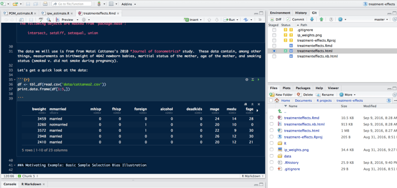
- Open the ‘treatmenteffects.RMD’ file and you will be able to run the chunks of code individually and walk through the estimation of i) Potential Outcome Means, ii) Inverse Probability Weighted Means, and iii) Propensity Score Adjusted Regression for the effect of smoking on birthweight problem from Cattaneo (2010).
You’ll notice the R Notebook, much like an R Markdown doc has code chunks marked by:
```{r}

```
but unlike your standard R Markdown doc you’ll notice a little play button in the top right corner of each code chunk.

Summary
- R Notebooks are pretty cool ways to combine text, equations, and interactive code
- They are a great tool for teaching, report generation, and collaborative coding
- Like regular R Markdown docs they can output to nice clean .html files or .pdf files…here is a sample from my Average Treatment Effects Notebooks output to .html and opened in a standard web-browser:
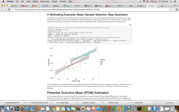
- Unlike regular R Markdown docs the code chunks in an R Notebook can be run independent of one another…so I user can monkey with options in one chunk and run it a few times without having to compile the entire document each time some code is run.
References
