
1st things first…data and code for the following exercises is up on GitHub:
https://github.com/aaronmams/treatment-effects
When it comes to estimating causal effects of treatments there are lot of ins and outs, a lot of whathaveyous, a lot of strands to keep in the ole duder’s head. Approaches like propensity score matching and difference-in-differences are used by (among others):
- economists to estimate things like the financial return on voluntary job training programs
- statisticians in the medical community to estimate treatment effects when randomized trials are not feasible (impact of smoking on birthweight of babies for example)
- political scientists to assess impacts of education on political participation
In my view, the causal treatment effects literature often gets confusing because different groups of people use different names for the same stuff.
I tried to attack this topic a few time before
- Here’s a post on Difference-in-Differences: https://thesamuelsoncondition.com/2016/04/14/difference-in-differences-primer/
- and here’s one on a related topic of natural expiriments and other stuff:
https://thesamuelsoncondition.com/2016/04/15/natural-experiments-in-public-policy-analysis/
This time I’m going to back up and try to add a little more meat to my previous mentions of sample selection bias.
——————————————————
Logistical Set-up:
I’m working with data containing birthweight observations on ~5,000 new borns. The data also have measurements on a number of characteristics of the mother.
- The data originally appeared in Matia Cattaneo’s 2010 study in the Journal of Econometrics
- The data are available for download here: http://www.stata-press.com/data/r13/te.html. They are labeled Cattaneo2.dta.
——————————————————–
——————————————————–
The Plan
Here’s what I’m going to discuss in this post:
1. Illustrative example of the selection-on-observables problem
2. Potential Outcome Means (POM) using regression adjustment
3. Inverse probability weight corrections (to the mean, and regression adjustment)
4. propensity score matching methods I decided not to do this one. I’ll shoot for an update next week where I get into matching models.
———————————————————
———————————————————
What is Selection on Observables?
Our data have, among other things, observations on baby’s birthweight, mother’s age, and an indicator for whether the mother smoked during pregnancy. We can consider ‘smoking during pregnancy’ to the treatment. When individual’s select into a treatment, the assignment to treatment and control can be nonrandom. That’s bad.
———————————————————
———————————————————
POM with Regression Adjustment
I don’t even really like this estimator but I came across a mention of it while reading up on inverse probability weights for sample selection corrections and it pissed me off….It pissed me off because all the discussions I read were extremely cryptic and it took me way longer than it should have to understand what the POM was/is. Since I hated the stuff I read, I figured I’d see if I can do better.
I came across the Potential Outcome Means (POM) while looking at some of functions in STATA’s ‘teffects’ suit of functions. There is a half-decent post about some of the treatment effect estimators on the STATA Blog here: http://blog.stata.com/2015/07/07/introduction-to-treatment-effects-in-stata-part-1/.
What I don’t like about this post is that it shows conceptually (graphically) what POM is and then it shows how to get the POM estimate (using regression adjustment) in STATA…They forgot to include the part where they actually tell us what, practically speaking, the POM estimator is.
Let’s imagine for a second that (all else equal) older mothers tend to give birth to heavier babies and smokers give birth to lighter babies but older mothers also tend to be smokers.
#generate some data to illustrate the potential observed mean
age=rnorm(100,30,5)
psmoke =  pnorm((age-mean(age))/sd(age))
smoke = rbinom(100,1,psmoke)
z = data.frame(age=age,smoke=smoke,bw=3000+(5*age)+(50*smoke) + rnorm(100,100,10))
Just to be really clear what we did there: we generated a probability of being a smoker which increased with age…more specifically it increases with higher positive departures from the mean age of the sample. Then whether the individual smokes or not was generated from a binomial distribution where the probability of success on a single trial was equal to the smoking probability (which increases with age).
From the perspective of estimating the effect of the treatment (smoking on birthweight) the ‘problem’ here is that we don’t have enough young women who are smokers (or enough older women who are non-smokers) to get a good estimate.
———————————————————
———————————————————
Potential Outcome Means (POM)
The POM estimator is really simple…so simple in fact that (if you’re like me) you may encounter a discussion of it out in the wild and assume that there is something you did not understand…because it sounds too simple to be legit. If it sounds too simple to work, then you probably understood it perfectly.
The POM estimator gets calculated like this:
- Estimate a linear regression for the sub-sample of smokers.
- Estimate a linear regression for the sub-sample of non-smokers.
- Using the full sample (smokers and non-smokers) get the fitted values using coefficients from #1.
- Using the full sample (smokers and non-smokers) get the fitted values using coefficients from #2.
You can do this pretty simply in R as follows:
#we are now switching over and using the Cattaneo birthweight data...I provided the link to those data above
#read the Cattaneo2.dta data set in
df = read.csv("/Users/aaronmamula/Documents/R projects/cattaneo2.csv")

#first fit the model using only the smokers
lm.smoker <- lm(bweight~mage,data=df[df$mbsmoke=='smoker',])
#get the fitted values using the entire data sample and the results from the
#'smoker' regression
pred.smoker <- predict(lm.smoker,newdata=df)
# get the mean predicted birthweight
mean(pred.smoker)

#next fit the model using only the non-smokers and follow
# the same steps as above
lm.ns <- lm(bweight~mage,data=df[df$mbsmoke!='smoker',])
pred.ns <- predict(lm.ns,newdata=df)
mean(pred.ns)
STATA apparently has a built-in procedure to do this:
teffects ra (bweight mage) (mbsmoke), pomeans
But if you compare the predicted means from the R code above to these results obtained using STATA’s fancy POM estimator, you’ll see they are identical.
One last thing we can do just to further our understanding of the POM estimator for average treatment effects is compare it the marginal effects estimated from a simple linear model:
#regress birthweight on age, smoker status and interaction term
bw.lm <- lm(bweight~mage+factor(mbsmoke)+factor(mbsmoke)*mage,data=df)
#get fitted values
df$pred.bw <- predict(bw.lm,newdata=df)
#compare mean fitted values for smokers and nonsmokers
mean(df$pred.bw[df$mbsmoke=='nonsmoker'])-mean(df$pred.bw[df$mbsmoke=='smoker'])
With the POM approach we get an -277.061 (smoking reduced the expected birthweight of babies by about -277 grams). With regular old OLS we get an estimated treatment effect of – 275.25.
In the data sample older women are more likely to be included and less likely to smoke…so without a sample selection correction we get a smaller estimated effect of smoking.
———————————————————————-
Inverse Probability Weight Adjustment
#start with the same fake data we used to illustrate the POM estimator
age=rnorm(100,30,5)
psmoke = pnorm((age-mean(age))/sd(age))
smoke = rbinom(100,1,psmoke)
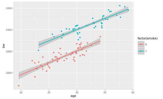
z = data.frame(age=age,smoke=smoke,bw=3000+(5*age)+(25*smoke) + rnorm(100,100,25))
ggplot(z,aes(x=age,y=bw,color=factor(smoke))) + geom_point() + geom_smooth(method='lm')
#calculate probability weights: fit a logit model and use the fitted values as
# probabilities
logit.bw = glm(smoke~age,data=z,family='binomial')
pi = predict(logit.bw,newdata=z,type="response")
#weight smokers by 1/p(i) so that weight is large when probability of being a smoker is
# small. Weight observations on non-smokers by 1/(1-p(i)) so weights are large when
# probability is small
z = tbl_df(z) %>% mutate(w=pi) %>%
mutate(weight=ifelse(smoke==1,1/pi,1/(1-pi)))
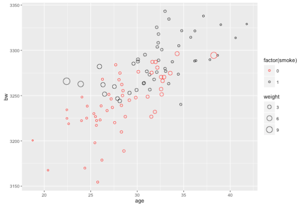
ggplot(z,aes(x=age,y=bw,color=factor(smoke),size=weight)) + geom_point(shape=1) + scale_color_manual(values=c("red","black"))
This plot will be a little hard to read but you should be able to get the gist: observations on smokers toward the younger end of the age range are weighted more heavily and observations on non-smokers toward the older end of the age range are weighted more heavily.
Ok, so switching over to the actual data, we will estimate the Average Treatment Effect using the inverse probability weights to take a weighted mean for the two groups:
#read the Cattaneo2.dta data set in
df = read.csv("data/cattaneo2.csv")

#use the probit link for probability weights like they do in the STATA blog
probit.bw = glm(mbsmoke~mage,data=df,family='binomial'(link='probit'))
pi = predict(probit.bw,newdata=df,type="response")

#add inverse probability weights to the data frame
df = tbl_df(df) %>% mutate(w=pi) %>% mutate(weight=ifelse(mbsmoke=='smoker',1/w,1/(1-w)),
                                             z=ifelse(mbsmoke=='smoker',1,0))

#ATE based on:
#http://onlinelibrary.wiley.com/doi/10.1002/sim.6607/epdf
weighted.mean.smoker = (1/(sum(df$z/df$w)))*sum(df$z*df$bweight/df$w)
weighted.mean.ns = (1/sum(((1-df$z)/(1-df$w))))*(sum(((1-df$z)*df$bweight)/(1-df$w)))

#ATE
weighted.mean.smoker - weighted.mean.ns
[1] -275.5007
Again, referring to the STATA blog we can confirm that our estimate of -275.5007 agrees with the estimate obtained using the less transparent STATA procedure:
teffects ipw (bweight) (mbsmoke mage, probit), ate
————————————————————–
The Inverse Probability Weight Regression Adjustment Estimator
Shit gets a little gnarlier at this point because the STATA blog introduces a lot of new covariates for the IPWRA. At this point I should also mention that my answers do match up with what you will find here and I’m not really sure why. I’ve spent a considerable amount of time trying to figure it out and frankly, I’ve given up.
The STATA folks aren’t that keen on telling you what their software does….if they did I suppose there is risk people wouldn’t keep paying them $2000/year for things that can be done in R and Python for free.
To be fair the STATA people aren’t the only offenders here. When I put, ‘Inverse probability weight regression adjustment’ into google scholar I got a bunch of biomedical research journal papers back. None of the top 12 papers on that list actually have an estimating equation written down in clear, arithmatic terms. They all says something like, “we used a logistic regression to derive the propensity score as the probability of receiving the treatment then adjusted the outcome model by inverse probability weights (Rosenbaum and Rubin, 1983).”
Rosenbaum and Rubin (1983) is a magnificent statistical treatise on average treatment effects…nowhere in it do they describe a technique as “regression adjustment with inverse probability weights.”
The ‘regression adjustment’ that I’m familiar with is a pretty vague term that generally means, “I added some more stuff to the right hand side of a regression in order to account for some confounders that might have been left out in the original regression.” A number of papers like this one support my interpretation of inverse probability weight regression adjustment as the following:
- we have an outcome
(perhaps birthweight of babies), two observable variables
(in the current context could be age and marital status), and a treatment variable
(smoker or non-smoker).
- we are worried that our estimate of the effect of age and smoking status on birthweight could be biased because we have a sample where younger mothers are also more likely to smoke…age is correlated with both the outcome variable and the assignment into treatment group.
- to ‘adjust’ our outcome model for this we first estimate the propensity score using a probit model:
- we use this model to get fitted values of the probability that individual
is a smoker given
and
,
.
- Now we include this propensity score as an ‘adjustment’ in a regression to determine the impact of smoking on birthweight,


This is a bit different (I think) from the prospect of using inverse probability weights to adjust a regression as they claim to do on the STATA blog…but honestly, I can’t really figure out what they did or how they did it…and nothing I’ve come across so far explains in any satisfactory level of technical detail what regression adjustment with inverse probability weights is.
Here is some code that will do my version of Propensity Score Regression Adjustment with a treatment models that includes all the variables used in the STATA blog example….If anybody wants to comment here or, even better, send a GitHub pull request and amend the code to show us how to do the STATA blog version of IPWRA that would be swell.
#read the Cattaneo2.dta data set in
df = read.csv("data/cattaneo2.csv")

#the treatment model
df = df %>% mutate(mage2=mage*mage) %>%
        mutate(marriedYN=ifelse(mmarried=='married',1,0),
               prenatal1YN=ifelse(prenatal1=='Yes',1,0))

ipwra.treat = glm(factor(mbsmoke)~mage+marriedYN+fbaby+mage2+medu,data=df,family='binomial'(link='probit'))
pi = predict(ipwra.treat,newdata=df,type="response")
df$ipwra.p = pi
df = df %>% mutate(ipwra.w=ifelse(mbsmoke=='smoker',1/ipwra.p,1/(1-ipwra.p)))

summary(lm(bweight~factor(mbsmoke)+ipwra.p,data=df))

Call:
lm(formula = bweight ~ factor(mbsmoke) + ipwra.p, data = df)

Residuals:
     Min       1Q   Median       3Q      Max
-3097.50  -315.07    23.65   353.62  2022.23

Coefficients:
                      Estimate Std. Error t value Pr(>|t|)
(Intercept)            3512.40      15.65 224.465  < 2e-16 ***
factor(mbsmoke)smoker  -224.84      22.26 -10.101  < 2e-16 ***
ipwra.p                -586.53      74.64  -7.858 4.82e-15 ***
---
Signif. codes:  0 ‘***’ 0.001 ‘**’ 0.01 ‘*’ 0.05 ‘.’ 0.1 ‘ ’ 1

Residual standard error: 565.2 on 4639 degrees of freedom
Multiple R-squared:  0.04695,	Adjusted R-squared:  0.04654
F-statistic: 114.3 on 2 and 4639 DF,  p-value: < 2.2e-16
If nothing else we can say we are moving in the right direction. The STATA blog has marginal impacts for smoking of:
- -277 for POM estimator
- -275 for the inverse probability weight adjustment to mean
- -229 for the IPWRA model
My results are identical for the first and second bullets and -224.84 for the third. So qualitatively at least my estimates are moving in the same direction as our STATA reference points.
