
I just finished writing a post breaking down some good, not so good, and downright dubious examples of public policy analysis I’ve seen recently in the scientific literature. I realized that, in the course of that post, I provided very little context on the types of empirical strategies that are often used in public policy analysis. Rather than go back and try to fit a quick primer on policy analysis methods into that, already crowded post, I thought I would try my hand at writing a few methods tutorials. I’m starting with a method that gets a lot of play in the type of policy analysis studies I like to read: Difference-in-Differences.
The classic motivating example for D-i-D analysis is here.
In the paper David Card and Alan Krueger evaluate the impact of a change in the minimum wage on employment. They use a sample of fast food restaurants (reasoning that if there is an employment effect to minimum wage changes it should certainly be visible among fast food firms, due to their heavy reliance on minimum wage labor) in New Jersey (a state that raised the minimum wage in April of 1992) and Pennsylvania (a neighboring state which did not experience a wage increase in April of 1992). In a nutshell, they found no discernible impact on fast food employment resulting from the increase in minimum wage. This study has become a bit controversial since, as you might imagine, some have used it to lobby for increases in state-wide minimum wages on the grounds that employment effects of such policies have been overstates. Conversely, others have attacked the study as flawed in attempts to counter the former groups lobbying efforts. I have no interest in weighing-in on the larger debate about minimum wages today. I’m just presenting this work as an example of public policy analysis that difference-in-differences can help inform.
Conceptual road-map
Suppose we are interested in the impact of a change in the minimum wage on employment. We could look at data from a state that changed their minimum wage at some time, 
Basically, when we use Difference-in-Differences we are looking for a way to separate out the observed change that we can attribute specifically to the policy change..versus all the other shit that makes things like employment go up and down.
Some more intuition
Employment in any particular restaurant in any particular state over time may go up or down because of
1. time-related effects – one way to think of these is overall macroeconomic changes that are causing changes to employment in every industry in every state,
2. region specific changes – independent of minimum wage policy, employment in a state may go up or down because of economic or policy changes (unrelated to minimum wage policy) at the state level…
Let’s think about two comparisons just to illustrate these issues.
Illustration 1
We have data on 50 fast food restaurants in two states (A and B) over 4 years. Following year 3, state A implements a minimum wage increase but state B does not.

Here, although we observe a decrease in average employment between years 3 and 4 in state A (the state that raised the minimum wage during this period), we see that average employment in state B exhibited similar trends. Here we would probably conclude that employment declines in the fast food industry in state A between years 3 and 4 are more likely to be the result industry-wide trends that are pushing fast food employment down in all states.
Illustration 2
Suppose we have data before and after the minimum wage change on employment by fast-food restaurants and some other industries that we don’t suspect would be affected by changes in the minimum wage. Suppose all our data is from the same state.
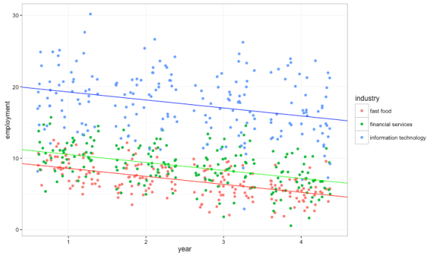
In the plot of totally made-up data above, the lines with colors corresponding to the colored points show mean employment in each industry.
Note that, although we did observe a decrease in employment in the fast food sector (the red line trending down) following the implementation of the minimum wage hike, the change appears consistent with the employment trends in broader economy.
Illustration 3
The two illustrations above were meant to drive home the point that assessing the impact of policy requires looking at relative changes. Illustrations 1 and 2 can kind of be thought of as ‘what might it look like if there were no change from the policy?”
We can contrast that with a ‘text book’ case of a policy induced shift, illustrated below.

In this case, State A implements a change in the minimum wage effective in year 3. State B does not. A foundational point with Difference-in-Difference analysis is that, if these two states are similar in most respects (such as neighboring states might be), then a good guess at what fast food employment would be in the absence of a change in the minimum wage can be constructed using fast food employment in the policy-unaffected state.
I think another illustration would be overkill here but it’s worth mentioning that, in addition to a level shift, we could think about a case where the trends (the slope of the two lines) were similar before the policy and completely divergent after the policy…think of two parallel lines before the policy that cross following the implementation of the policy.
Econometric Estimation of a DiD Model
In Card and Krueger’s (1994) study of the impact of a change in the minimum wage on employment in wage-dependent industries, they collected data from a sample of fast food restaurants in New Jersey and Pennsylvania. In April of 1992 the minimum wage in New Jersey increased from $4.25/hour to $5.05/hour. The minimum wage in neighboring Pennsylvania did not change.
Card and Krueger collected wage and employment data, along with other characteristics, of 410 fast food restaurants in NJ and PA at two points in time: first during the period Feb-March of 1992 (just before the minimum wage increase) and then again in Nov-Dec of 1992 (about 8 months after the wage increase). As discussed above, by comparing the treatment group (NJ, the state that enacted the wage increase) with the control (PA which, as a neighboring state, is presumed to be similar to NJ in many respects except it did not receive the treatment…i.e. there was no change in the minimum wage) we can isolate the marginal impact of the wage increase on fast food employment.
I downloaded the data used for this study here
First, let’s consider a model with a pretty simple additive structure. In our data we have:
- 384 restaurants (the original sample has 410 but 26 are missing at least one of the employment categories needed to calculate full time equivalent employment in both periods).
- 2 states, call them
for the policy affected state and
for the policy unaffected state.
- 2 time periods, call them
and
.
is the number of full time equivalent employees in restaurant
, in state
, in time
.
- let
be a dummy variable such that
if
if
- let
be a dummy variable such that
if the restaurant is in the policy unaffected state (PA) and
if the restaurant is in the policy affected state (NJ).
With this set-up we could write the following model:

Here,
captures state-specific variation
capture year-specific variation
- The interaction term
will equal 1 in the policy-affected area and 0 otherwise…this captures our marginal employment effect of being in the affected state after the policy.
In this model, the change in expected value of employment in the affected area from the first to the second period is:

And the change in expected value of employment in the policy unaffected state is,

So we have,

showing that the DiD estimator (
require(dplyr)
require(ggplot2)
#------------------------------------------------------
#DiD Example 4 - replicate Card and Krueger's 1994
#  minimum wage study

#read in data provided by Guido Imbens...note that in Card and Krueger's original
# study they define full time equivilent employees to be full time employees +
# managers + 0.5 * part-time employees

#in the data set the following columns are combined to create the variable
# full time equivilent employees:

# empft - the number of full time employees before the wage increase
# emptf2 - the number of full time employees after the wage increase
# emppt - the number of part time employees before the wage increase
# emppt2 - the number of part time employees after the wage increase
# nmgrs - the number of managers before the wage increase
# nmgrs2 - the number of managers after the wage increase

njmin = tbl_df(read.csv("/Users/aaronmamula/Documents/R projects/njmin.csv")) %>%
  mutate(delta=(empft2+emppt2) - (empft+emppt),fte=nmgrs+empft+(0.5*emppt),
         fte2=nmgrs2+empft2+(0.5*emppt2))

#quick calculation of means to make sure our data line up with whats in
# the paper
njmin %>% group_by(state) %>% summarise(mean_fte=mean(fte,na.rm=T),
                                      mean_ft2=mean(fte2,na.rm=T))
#we can compare these numbers to Table 2 from Card and Krueger (1994) and
# confirm that we are working with the same data
#-------------------------------------------------------

#------------------------------------------------------
# set up the data for DiD estimation, not completely necessary
# but I'm used to the dplyr/ggplot environment that prefers data
# in long format
est.df = tbl_df(rbind(data.frame(sheet=njmin$sheet,chain=njmin$chain,
                                  state=njmin$state,emp=njmin$fte,t=0),
                 data.frame(sheet=njmin$sheet,chain=njmin$chain,
                            state=njmin$state,emp=njmin$fte2,t=1)))

#here state=0 is PA and state=1 is NJ; we set t = 0,1 so we can interact these
# directly to get the DiD coefficient...using the OLS estimator with lm()
# gives up the DiD estimate
summary(lm(emp~factor(state) + factor(t) + (state:t),data=est.df))
#------------------------------------------------------
We can compare the means in the data above to Table 2 from Card and Krueger (1994) and confirm that we are working with the same data.
In the final line above we estimate the model. Note that the estimated coefficient on the interaction of state*time is 2.754 and is marginally significant. This matches the change in mean FTE employment reported in Card and Krueger’s Table 3, row 3.
Two important points to mention before closing this out:
- There are a few different empirical specifications in the Card and Krueger paper. I’m not going to try and replicate them all but you all should be aware that the authors did consider some complicating factors such as the fact that not all restaurants in the sample in NJ were initially paying the $4.25 minimum wage…some were actually paying a $5.00 wage before the minimum wage hike took effect. I highly recommend reading the original papers and the many follow-ups that it spawned.
- It’s also probably worth reading the Bertrand, Duflo and Mullainathan paper, How Much Should We Trust Difference-in-Difference Estimates?. Despite it’s alarmist title, it turns out the answer is, “A lot.. as long as you use robust standard error estimates, DiD estimates are quite trustworthy.”
- A more general final point: DiD estimation can be very satisfying in cases where a treatment/control set-up is intuitive…such as comparing fast food employment in a state that enacted a minimum wage hike with fast food employment in a neighboring state that did not change the minimum wage. There are many policy settings (like state-by-state health policy changes) where we would like to know the marginal impact of the change but there are no intuitively obvious policy unaffected control groups (more often than not what we have in these situations is different groups that we suspect have different levels of exposure to the policy). Maybe I’ll flush this issue out in another post but, for now, if you are interested in DiD and more generally interested in the full panoply of options available for empirical policy evaluation, you might want to Google ‘dynamic panel models’ and ‘propensity score matching.’
