
Yesterday I tried to squeeze two related but complicated topics into the same post…I fear it did not go well. After a little more tinkering I think I’ve made substantial improvements to the R Markdown section of yesterday’s post.
If you didn’t make it all the way through yesterday’s post I don’t blame you and I won’t make you read it just to get up to speed. Here is what you need to know:
- I have a data set that contains the value of a stock trading portfolio on each day from 2013-11-11 to 2016-05-16. The data also include some documentation on every trade made in that account. For reasons I don’t want to fully get into right now those data are contained in .csv file named ‘changes.csv’
- At the end of each week, I want a report on all the changes (new purchases of stock, new stock shorts, any sale of shares) to the account.
- Because the process is dynamic (each week new data is added when new positions are opened or old positions are closed) I’m going to use R Markdown to build a template for my report. Then each week, I can generate the same report for the current week by simply changing a few parameters.
The basic attraction of R Markdown is that I can embed R code into a text-like document and, when the document is compiled, the embedded R code will be run and the document will get updated.
The current use-case utility is this:
- Inside the R Markdown document the data from ‘changes.csv’ are read-in as a data frame.
- The relevant parameters are the current week and year
- The code embedded in the R Markdown doc take the value for week and year, pull data from the data frame for the relevant week and year, and output a set of tables that describe each position that changed for that week.
An example will probably help clarify things:
---
title: Weekly Transaction Report
author: aaron mamula
date: June 3, 2016
output: html_document
---

```{r, include=FALSE}
library(dplyr)
library(ggplot2)
changes = tbl_df(read.csv('changes.csv'))  %>% mutate(date=as.Date(date))

head(changes)

```

```{r,include=FALSE}
wk=46
yr=2013
wk.start=min(changes$date[changes$week==wk & changes$year==yr])
wk.end=max(changes$date[changes$week==wk & changes$year==yr])
```

##Transaction Log for week `r wk`: `r wk.start` to `r wk.end`

```{r, echo=FALSE}

position.sum.wk = function(wk,yr){
#generate a list of asset names for positions that changes this week
tradeids = changes$id[changes$week==wk & changes$year==yr & changes$diff!=0 &
                         changes$asset!='CASH'& is.na(changes$diff)==F]
history.fn = function(tid){
 t.date = changes$date[changes$id==tid]
    a = changes$asset[changes$id==tid]
    hist.df = changes[changes$date<t.date & changes$asset==a,]
   #find he latest date in the data frame for which the position was 0
    pos0 = max(hist.df$date[hist.df$shares==0])
      hist.df = changes %>%
      filter(changes$date>= pos0 & changes$date<=t.date & asset==a) %>%
        select(shares,asset,date,costbasis,saleprice,Close,diff)
  names(hist.df) = c('open position','asset','date','costbasis','saleprice','Close','diff')
return(hist.df)
}
lapply(tradeids,history.fn)
}

```

```{r,include=FALSE}
dlist=position.sum.wk(wk=wk,yr=yr)
```

```{r,echo=FALSE}
lapply(c(1:length(dlist),function(i){
  x = dlist[[i]]
  a = unique(dlist[[i]]$asset)
  y = knitr::kable(x, digits = 2, col.names=c('open','asset','date','cost basis','sale price','close','diff'),caption = paste('position change',a))
  return(y)
})

```
This code, when knitted, produces the following html doc:
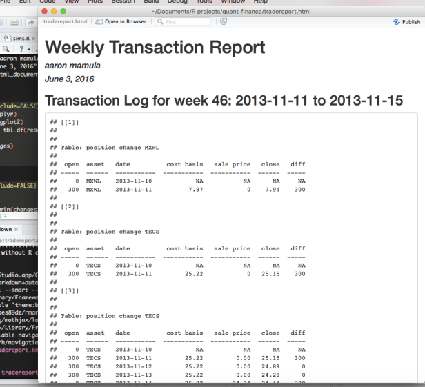
Just to make sure we are on the same page with respect to what I’m trying to do, notice that the first table in the html doc that is output from R Markdown has two rows related to the asset ‘MXWL.’ It says that on 2013-11-10 we owned 0 shares of ‘MXWL’ and on ‘2013-11-11’ we owned 300 shares. That is, we purchased 300 shares of Maxwell Technologies on 2013-11-11. The second table indicated that on the same day, 2013-11-11, we purchased 300 shares of TECS. The third table indicates that on 2013-11-14 we sold 300 shares of TECS and the table give us the complete history of that position that was closed out on 2013-11-14.
A few things to note about the R Markdown:
1. In R Markdown we specify that R code is about to be supplied by using the syntax:
`r rcodehere`
If we want to specify a code chunk we may use
“`{r}
r code line 1
r code line 2
“`
As a very simple example, if I had a data frame read into an R Markdown document with 10 rows and 3 column and the data frame were named mydata, I could output the statement, “The data frame mydata has 10 rows and 3 columns” by writing:
The data frame mydata has `r nrow(mydata)` and `r ncol(mydata)`
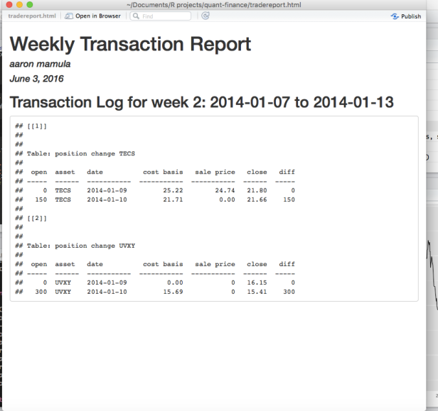
2. The key thing we discussed yesterday was that the function ‘position.sum.wk’ accepts the input arguments ‘wk’ and ‘yr’. The dynamic documents part of R Markdown is that I can change only these two arguments and generate a new report identical to the report above but for a different week and year:
---
title: Weekly Transaction Report
author: aaron mamula
date: June 3, 2016
output: html_document
---

```{r, include=FALSE}
library(dplyr)
library(ggplot2)
changes = tbl_df(read.csv('changes.csv'))  %>% mutate(date=as.Date(date))

head(changes)

```

```{r,include=FALSE}
wk=2
yr=2014
wk.start=min(changes$date[changes$week==wk & changes$year==yr])
wk.end=max(changes$date[changes$week==wk & changes$year==yr])
```

##Transaction Log for week `r wk`: `r wk.start` to `r wk.end`

```{r, echo=FALSE}

position.sum.wk = function(wk,yr){
#generate a list of asset names for positions that changes this week
tradeids = changes$id[changes$week==wk & changes$year==yr & changes$diff!=0 &
                         changes$asset!='CASH'& is.na(changes$diff)==F]
history.fn =function(tid){
 t.date = changes$date[changes$id==tid]
    a = changes$asset[changes$id==tid]
    hist.df = changes[changes$date<t.date & changes$asset==a,]
   #find he latest date in the data frame for which the position was 0
    pos0 = max(hist.df$date[hist.df$shares==0])
      hist.df = changes %>%
      filter(changes$date>= pos0 & changes$date<=t.date & asset==a) %>%
        select(shares,asset,date,costbasis,saleprice,Close,diff)
  names(hist.df) = c('open position','asset','date','costbasis','saleprice','Close','diff')
return(hist.df)
}
lapply(tradeids,history.fn)
}

```

```{r,include=FALSE}
dlist=position.sum.wk(wk=wk,yr=yr)
```

```{r,echo=FALSE}
lapply(c(1:length(dlist)),function(i){
  x = dlist[[i]]
  a = unique(dlist[[i]]$asset)
  y = knitr::kable(x, digits = 2, col.names=c('open','asset','date','cost basis','sale price','close','diff'),caption = paste('position change',a))
  return(y)
})

```
The key innovations over yesterday’s post are twofold:
1. In the code I posted yesterday each output table was generated by a separate code block. The problem with this is that each week there will be a different number of total changes to positions within the portfolio. That means that if the output tables are generated by their own code we need to know how many position changes there are for the current week and change the code accordingly.
In the new code, I have replaced explicit table generation with a single code block that sniffs out the total number of position changes in the current week and creates a table for each position change. Refer to the ‘lapply’ statement beginning on line 54 in the code block above to see how the tables are not dynamically generated.
2. I discovered that the package ‘kable’, with pretty minimal time investment, can really sex-up the look of output tables in R Markdown. I’ll freely admit that I don’t totally understand how this works since, when I tried to install the package ‘kable’ and ‘printr’ through the console I was told that they are not available for R 3.3.3…but they seem to work ok when I call them through R Markdown.
I plan to keep tinkering…I’ll let you know if any other marginal improvements arise.
