Starting with this post I laid out the motivation for my recently renewed interest in time-series analysis. To recap, my basic motivating question is, “what do I do if I’m modeling a process I suspect is seasonal (monthly landings in a commercial fishery for example) but I also have reason to suspect the nature of seasonality might be changing?”
To be a bit more specific here, I’m dealing with several years worth of data on total monthly catches by a group of fishermen. The data exhibit some seasonal signals with catches tending to be higher in the summer and early fall and lower in the late fall, winter, and early spring. I observe that a particular regulation went into effect in year 

In my reading of the literature I determined I have two intellectual paradigms to choose from:
- Smooth transition/regime change models
- Markov Regime Switching Models, ala Hamilton 1989 and many others.
- Smooth transition regressions
- Change-point detection models including
- identification and dating of unknown structural breaks
- Bayesian change point models
The conceptual difference between items #1 and #2 hinges on whether you are
- dealing with a process that moves back and forth between a finite number of states (and the process behaves differently in each state)
- the canonical example here is a macro-economic time-series that may have a different mean and variance depending on whether we are in an expansionary or contractionary phase of the business cycle.
- dealing with a process that, once it departs from its past behavior at some point in the time-series, never returns to exhibit similar properties as before.
- an example I’ve seen used here is the demand for red meat and poultry among American consumers around the 1970s. Somewhere in this time the relationship between demand for these two products was fundamentally and permanently altered as consumers became more health conscious. The implication being that the time-series here can really be modeled as two completely different series: those observations before 1978 and those observations after 1978.
In the interest of keeping this a little bit concise and digestible I’m going to, for the moment, abstract away from the discussion about how one decides on the right modeling approach and just focus on how to implement these approaches (I’ll circle back to the issue of which approach is the right on in a future post….maybe Time-series VII or VIII).
I’m going to start with the Markov Regime Switching Model because its one I’ve worked with before and I’m at least a little familiar with it. My first goal – the one I will focus on in this post – is just to understand the basic mechanics and properties of Markov Regime Switching Models.
#################################################################
#################################################################
#################################################################
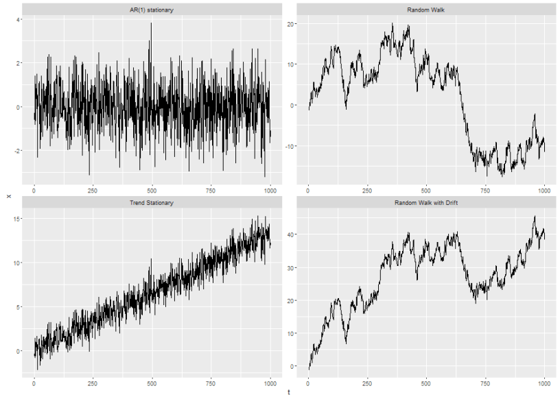
First, a picture…because I really like pictures. Goldfeld and Quandt (1973), Hamilton (1989) and a bunch of other really smart dudes observed that certain macro-economic time-series like the unemployment rate, federal funds rate, new housing starts, etc. seem to behave differently depending on whether the economy is in an expansionary or contractionary phase.
To illustrate what this might look like, it’s not hard to image a financial asset that is more volatile during market downturns and less volatile during bull markets. Let 
If we were to generate data from the following process:


and we define periods 1-10, 16-30, and 40-60 to be in regime 1…we might produce something like this:

#################################################################
#################################################################
#################################################################
#################################################################
#################################################################
#################################################################
Ok, so now that we’ve seen what a Markov Regime Switching Process might look like, let’s run through the discount version of what a Markov Regime Switching Model is….I can’t really improve on the many tutorials already out there so I’ll try to keep this brief:
I’m cribbing heavily from one of Erik Kole’s examples because I find it very clear. Suppose we have data on financial returns of a particular asset (call this 


Call this ‘state of the economy’ process the regime and let 

The return

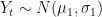
So 


The kicker here is that we don’t directly observe the regime in time
![\xi_{jt}=Pr[S_{t}=j|\Omega_{t};\theta]](https://s0.wp.com/latex.php?latex=%5Cxi_%7Bjt%7D%3DPr%5BS_%7Bt%7D%3Dj%7C%5COmega_%7Bt%7D%3B%5Ctheta%5D&bg=%23ffffff&fg=%23111111&s=0&c=20201002)
where 
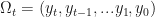

In this case we are assuming the unobserved state (regime) follows a Markov Process – meaning that all the information we need to predict next period’s value is contained in last period’s value. So now we introduce the regime-transition parameters. Let:
![p_{ij}=Pr[S_{t}=i|S_{t-1}=j]](https://s0.wp.com/latex.php?latex=p_%7Bij%7D%3DPr%5BS_%7Bt%7D%3Di%7CS_%7Bt-1%7D%3Dj%5D&bg=%23ffffff&fg=%23111111&s=0&c=20201002)
The probability model for the unobserved state can now be formed using Bayes’ Rule:
![P[S_{t}=0|Y_{t}=y_{t};\theta]=\frac{P[Y_{t}=y_{t}|S_{t}=0]P[S_{t}=0]}{Pr[Y_{t}=y_{t}]}](https://s0.wp.com/latex.php?latex=P%5BS_%7Bt%7D%3D0%7CY_%7Bt%7D%3Dy_%7Bt%7D%3B%5Ctheta%5D%3D%5Cfrac%7BP%5BY_%7Bt%7D%3Dy_%7Bt%7D%7CS_%7Bt%7D%3D0%5DP%5BS_%7Bt%7D%3D0%5D%7D%7BPr%5BY_%7Bt%7D%3Dy_%7Bt%7D%5D%7D&bg=%23ffffff&fg=%23111111&s=0&c=20201002)
Here, it is worth highlighting a few things:
1.
![Pr[S_{t}=0]=Pr[S_{t-1}=0]*p_{00} + Pr[S_{t-1}=1]*(1-p_{11})](https://s0.wp.com/latex.php?latex=Pr%5BS_%7Bt%7D%3D0%5D%3DPr%5BS_%7Bt-1%7D%3D0%5D%2Ap_%7B00%7D+%2B+Pr%5BS_%7Bt-1%7D%3D1%5D%2A%281-p_%7B11%7D%29&bg=%23ffffff&fg=%23111111&s=0&c=20201002)
That is, once inference has been made about the probability of being in each of the two regimes in time
2. ![Pr[Y_{t}=y_{t}|S_{t}=0]=f(y_{t}|S_{t}=0,\Omega{t-1};\theta)=\frac{1}{(2 \pi \sigma_{0}^{2})^{0.5}}exp[\frac{1}{2 \sigma_{0}^{2}}(-(y_{t}-\mu_{0})^{2})]](https://s0.wp.com/latex.php?latex=Pr%5BY_%7Bt%7D%3Dy_%7Bt%7D%7CS_%7Bt%7D%3D0%5D%3Df%28y_%7Bt%7D%7CS_%7Bt%7D%3D0%2C%5COmega%7Bt-1%7D%3B%5Ctheta%29%3D%5Cfrac%7B1%7D%7B%282+%5Cpi+%5Csigma_%7B0%7D%5E%7B2%7D%29%5E%7B0.5%7D%7Dexp%5B%5Cfrac%7B1%7D%7B2+%5Csigma_%7B0%7D%5E%7B2%7D%7D%28-%28y_%7Bt%7D-%5Cmu_%7B0%7D%29%5E%7B2%7D%29%5D&bg=%23ffffff&fg=%23111111&s=0&c=20201002)
The conditional density of Y given the current regime, past information, and parameter vector is normal with parameters 
We can do a couple things to represent this a little more compactly:
First, let
P=
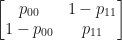
and let,
![Pr[S_{t}=j|\Omega_{t};\theta]=\xi_{t|t}=\begin{pmatrix}\ \xi_{0t}\\ \xi_{1t}\end{pmatrix}](https://s0.wp.com/latex.php?latex=Pr%5BS_%7Bt%7D%3Dj%7C%5COmega_%7Bt%7D%3B%5Ctheta%5D%3D%5Cxi_%7Bt%7Ct%7D%3D%5Cbegin%7Bpmatrix%7D%5C+%5Cxi_%7B0t%7D%5C%5C+%5Cxi_%7B1t%7D%5Cend%7Bpmatrix%7D&bg=%23ffffff&fg=%23111111&s=0&c=20201002)
finally, denote

Now the series of inference and forecast probabilities regarding the unobserved state (regime) that we need can be expressed as,


This probability model can be solved for the optimal values of ![\theta=[\mu_{0},\sigma_{0},\mu_{1},\sigma_{1},p_{11},p_{22}]](https://s0.wp.com/latex.php?latex=%5Ctheta%3D%5B%5Cmu_%7B0%7D%2C%5Csigma_%7B0%7D%2C%5Cmu_%7B1%7D%2C%5Csigma_%7B1%7D%2Cp_%7B11%7D%2Cp_%7B22%7D%5D&bg=%23ffffff&fg=%23111111&s=0&c=20201002)
![L(y_{1},y_{2},...y_{T};\theta)=\Pi_{t=1}^{T}Pr[Y_{t}=y_{t}|\Omega_{t-1};\theta]](https://s0.wp.com/latex.php?latex=L%28y_%7B1%7D%2Cy_%7B2%7D%2C...y_%7BT%7D%3B%5Ctheta%29%3D%5CPi_%7Bt%3D1%7D%5E%7BT%7DPr%5BY_%7Bt%7D%3Dy_%7Bt%7D%7C%5COmega_%7Bt-1%7D%3B%5Ctheta%5D&bg=%23ffffff&fg=%23111111&s=0&c=20201002)
and noting that ![Pr[Y_{t}=y_{t}|\Omega_{t-1};\theta]=\xi_{t|t-1}'f_{t}](https://s0.wp.com/latex.php?latex=Pr%5BY_%7Bt%7D%3Dy_%7Bt%7D%7C%5COmega_%7Bt-1%7D%3B%5Ctheta%5D%3D%5Cxi_%7Bt%7Ct-1%7D%27f_%7Bt%7D&bg=%23ffffff&fg=%23111111&s=0&c=20201002)

A popular way to maximize this function for optimal parameter values is through the use of the Hamilton Filter. I’ll post some code for that tomorrow.
#################################################################
#################################################################
#################################################################
