
I’m working on getting all the code for this chunk of posts on time-series analysis up on GitHub…it’s not there yet but maybe by the end of the day.
This post is going to be short because I don’t really think I can add much value to what is already out there and easily accessible on autocorrelation in time-series data.
- a really nice tutorial (a bit advance) complete with a lot of R code exists here.
- the best semi-technical but very accessible reference I know is Peter Kennedy’s Guide to Econometrics
I’m doing this primarily so that my little mini-treatise on time-series will be self-contained. Remember that I’m really hoping to get to sometime soon is talking about how to approach a seasonal time-series when we think the seasonality is changing (either in an evolutionary sort of way or in a discrete structural break sort of way). To do that, I need to draw on basic time-series concepts like autocorrelation/serial correlation of residuals…and so I want these things laid out in posts that I can draw on later.
Most economic treatments of time-series approach autocorrelation in regression residuals as a problem that needs to be fixed. Basically, if you have a regression model:

and
![E[\epsilon_{t}\epsilon_{r}] \neq 0, t\neq r](https://s0.wp.com/latex.php?latex=E%5B%5Cepsilon_%7Bt%7D%5Cepsilon_%7Br%7D%5D+%5Cneq+0%2C+t%5Cneq+r&bg=%23ffffff&fg=%23111111&s=0&c=20201002)
then the ordinary least squares estimator is no longer Best Linear Unbiased.
I’m not wild about this starting point for talking about error correlation because I don’t feel the need to force every problem into an OLS framework…I’m perfectly happy applying non-linear or biased model when the situation calls for them.
Even though I don’t do a lot of pure prediction type analysis, I actually kind of like the prediction error rational for motivating a discussion of autocorrelated residuals. Basically, if you have a model where the errors are autocorrelated it can mean that overprediction of 

Ok, so what does it look like when you have autocorrelated errors? Let’s revisit our AR(1) process with trend from this post:
set.seed(1)
x.trend <- w.trend <- rnorm(120)
for (t in 2:120)x.trend[t] <- (x.trend[t-1]*0.25)+w.trend[t] + 0.1*t
tmp <- data.frame(t=c(1:120),x=x.trend)
ggplot(tmp,aes(x=t,y=x)) + geom_line() + stat_smooth(method='lm')
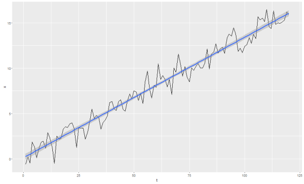
Now let’s say we model this with a simple linear time trend. That is, we estimate 

using OLS.
tmp$pred <- lm(x~t,data=tmp)$fitted.values
tmp$error <- tmp$x-tmp$pred
We want to know if the errors are correlated in time. I’ll do this by hand first for illustrative purposes, then we’ll do a couple formal tests on our real seasonal data.
First, test for significant correlation between 

#are the errors correlated
tmp <- tbl_df(tmp) %>% mutate(e1=lag(error))
cor.test(tmp$error[2:nrow(tmp)],tmp$e1[2:nrow(tmp)])

	Pearson's product-moment correlation

data:  tmp$error[2:nrow(tmp)] and tmp$e1[2:nrow(tmp)]
t = 2.6624, df = 117, p-value = 0.00885
alternative hypothesis: true correlation is not equal to 0
95 percent confidence interval:
 0.06166282 0.40171924
sample estimates:
      cor
0.2390056
This suggests that our errors are positively and significantly correlated.
Now a ghetto runs test. A runs test basically tries to evaluate whether positive errors tend to be followed by positive error and negative errors tend to be followed by negative errors.
#ghetto runs test...are positive values followed by positive values? tmp <- tmp %>% mutate(run=ifelse(error&gt;0,1,ifelse(error==0,0,-1))) ggplot(tmp,aes(x=t,y=run)) + geom_line()
It’s worth mentioning that most statisticians prefer the Q-Q plot of some other test of normality in conceptualizing correlated errors…I just went with a jerry-rigged runs test because I think it paints a nice picture:
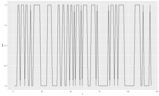
those little horizontal segments where the series is at +1 for a while or at -1 for a while…those, in the words of the great Jeff Foxworthy are very much bad.
So far, so good. Now let’s quickly cover some more formal tests and put this topic to bed. Here I’m going to focus on the second series that was generated (the series with seasonality throughout) and further, I’m going to focus only on the portion before the structural break that I induced.
Here is what we are going to do:
- generate a seasonal (monthly) process
- estimate a linear model with monthly dummy variable
- test this model for serial correlation in the errors
IMPORTANT NOTE: I’m including the data generation step for the following reason: the process doesn’t have much error in it. That means that any small anamolies can impact the results a lot. This process shouldn’t have serial correlation in the residuals of the model. That is because, once we control for the season (month) by including the monthly dummy variable, there should no additional information to be gained by including lagged terms in the model. The effect of month is constant across all years in the series. However, in practice, I noticed that 1 or 2 out of every 10 series I generated had some small random disturbance that gave it the appearance of autocorrelation. So I’m including the data generation part here so you can satisfy yourselves that most series generated with my code should not have autocorrelated residuals in the monthly dummy variable regression.
df.tmp <- seasonal.data(sigma1=10,sigma2=100,nmonth1=72)
df.tmp <- df.tmp[which(df.tmp$series==2 & df.tmp$year<2011),]
mod.pre <- lm(lbs~feb+mar+apr+may+jun+jul+aug+sep+oct+nov+dec,
          data=df.tmp)
df.tmp$resid <- mod.pre$residuals
df.tmp$fitted <- mod.pre$fitted.values
The formal test we will use here is theBreusch Godfrey Test for serial correlation in the errors. Note that one often sees plots of the autocorrelation function and partial autocorrelation functions presented as a first, visual, step towards diagnosing autocorrelation. I’m skipping this step because I prefer the ACF and PACF diagnotics for addressing things like, “How many lags should I include in my ARMA model?” or “is my data seasonal?” I already know the data are seasonal because I made them…and I’m trying to focus on a slightly different (although admittedly related) question here, “Is my seasonal dummy variable regression any good?”
The Breusch-Godfrey test is available in R as part of the lmtest package…but it’s just as easy to DIY so let’s do that:
In a linear regression of the form,

residuals of the model might correlated through time such that

Breusch and Godfrey showed that using the residuals from the original regression and performing the auxiliary regression,

will produce an 
So, now all that remains to be done is:
- Run the regression using monthly dummy variables as predictors for pounds landed…actually I’ve already done this above, the results are saved in the object mod.pre
- get the residuals from that model…again, this step was done above and these residuals now live in the data frame as df.tmp$resid.
- created p lags of the residual. I’m going to use p = 12 because I have a monthly process so I want to make sure to test for serial correlation all the way up to the 12th order lag
- run a regression of the residuals on all variables from the original regression plus the p lagged residual terms.
- recover the
. If this value is less than the critical value (18.54 for
and significance level = 90%).
#now create the lagged residuals for the BG test
df.tmp <- df.tmp %>% mutate(r1=lag(resid,1),r2=lag(resid,2),
r3=lag(resid,3),r4=lag(resid,4),
r5=lag(resid,5),r6=lag(resid,6),
r7=lag(resid,7),r8=lag(resid,8),
r9=lag(resid,9),r10=lag(resid,10),
r11=lag(resid,11),r12=lag(resid,12))
BG.test <- lm(resid~feb+mar+apr+may+jun+jul+aug+sep+oct+nov+dec+r1+
r2+r3+r4+r5+r6+r7+r8+r9+r10+r11+r12,data=df.tmp)
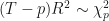
#the relevant test statistic is:
# (T-p)*R^2
# which is distributed approximately Chi-Squared(p) and test the null
# hypothesis that all rho = 0 (no autocorrelation)
BG.teststat <- (nrow(df.tmp)-12)*summary(BG.test)$r.squared
#chi-square critical values for p=12 (number of regressors in the model)
# degrees of freedom is 18.5 for alpha = 0.9
BG.teststat
9.205
