
This is a follow-up on my last two posts that dealt with methods used by social scientists to quantify impacts of public policy choices.
My primary motivation for penning a few words on these two methods/approaches was that I gave them some lip-service in my critique of the fluffy data analysis in the book Zillow Talk. I felt bad for just dropping a quick, “they should have used difference-in-differences” then moving on…so I decided to rectify that with some longer posts.
This is the final installment of the little mini-series that I’m calling (in my head at least) some stuff you should know about if you want to do policy analysis.
The first installment was a primer on Difference-in-Difference estimation is here.
Related to D-i-D, the second post was a little discussion of natural experiments and how they can help us isolate the true impact of a policy change is here.
This final post will deal with an emerging topic in public policy analysis: Synthetic Controls.
Here’s the outline:
- Synthetic Control: what’s the elevator pitch?
- What’s it used for?
- Why do people like it?
- A little math
- A quick intro to the R package ‘Synth’
Synthetic Control: the elevator pitch
With the Difference-in-Differences studies that I linked to previously, we look at treatment/control set ups where one unit was affected by a policy change, other units were not, and outcomes between the affected and unaffected units before and after the change were compared. Synthetic Control takes a similar general approach but, instead of relying on one unaffected unit or the average across many unaffected units to create the counterfactual, Synthetic Control uses a linear combination of unaffected units to create a hypothetical unit that bears the closest possible resemblance to the affected unit.
What is Synthetic Control Used for?
Short answer is basically the same stuff that Difference-in-Differences or other observational policy analysis methods are used for.
- Abadie, Diamond, and Hainmueller developed the method and used it evaluate the effect of California’s 1988 anti-tobacco policies on smoking rates. In a nutshell, this study looked at how cigarette consumption per capita evolved in California before and after implementation of a large scale anti-tobacco initiative…and how that compared to states that did not implement anti-tobacco measures.
- Munasib and Rickman used it to evaluate the effect of unconventional oil and gas exploration (fracking) on employment and income in non-metropolitan (rural) counties.
- In an intensely interesting paper I read this morning, Billmeier and Nannicini used it to assess the impact of economic liberalization (trade openess mainly) on a country’s GDP per capita.
Why do people like it
Abaide et al. identify three main features that they highlight as strengths of the Synthetic Control approach. I was moved by one in particular:
In traditional treatment/control type observational studies, the control units can be chosen in a pretty ad-hoc manner. If we want to evaluate the impact of a fracking boom on income and employment we could feel pretty good about comparing North Dakota and South Dakota (two highly rural states with a few population centers and similar economic make-up as regards major industries). And we could be somewhat certain that we don’t want to compare North Dakota with New Jersey (not similar in size, economic make-up, little geophysical similarity, etc.). But what about Nebraska? or Utah? Point being, there is some grey area. Synthetic Control addresses this by quantifying the similarity between affected and unaffected units in order to minimize the difference between treatment and control.
As they state in the paper:
Because synthetic control is a weighted average of the available control units, the synthetic control method makes explicit: (1) the relative contribution of each control unit to the counterfactual of interest; and (2) the similarities (or lack thereof) between the unit affected by the event or intervention of interest and the synthetic control, in terms of preintervention outcomes and other predictors of post-intervention outcomes…
A little math
I don’t want to get bogged down in this…but math (for those that are comfortable reading it) lends itself to concise explanation of things that would take a lot of space and vocabulary to explain in words.
My interpretation of the kernel of info we need in order to understand synthetic controls is as follows:
Suppose, like Abaide, Diamond, and Hainmueller, we have per capita consumption of cigarettes (Y) for several years before and several years after the policy change.
-
is the outcome that would be observed for state
in the absence of the policy.
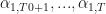
-
is the number of pre-intervention time periods
-
is the outcome that would be observed for state
to

The intervention has no effect on the states before implementation so:

for 
Next, define 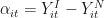

Without loss of generality, assume that the policy affected state is state 1. What we are interested in is,
For 

Because state 1 is the exposed unit we observe 


Let,

with
-
unknown year controls common across all units$
-
are observed covariates not affected by the intervention and
parameters
-
are unobserved common factors
-
unknown factor loadings
Let there by 


Each particular 

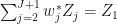
The value of the outcome variable for each synthetic control is,

Ok, here is the meat of the matter:
suppose there are 
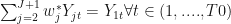
and
Under fairly general conditions, Abadie et al. show that with these 

Abadie et al. actually go a step further and show that as long as


holds approximately, that

Implementation
To recap, if we can find 

The issue now is finding the weights.
Start by considering a particular linear combination of the outcome variables denoted,

Here,

The subscript 
What this means in the following:
think about a particular 


Then 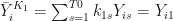
We could also define a 

and the resulting

From these two examples it’s probably clear that there are many possibilities for the 
We will consider:
-
possible linear combinations of the outcome variables
-
variables in the vector
-


Now define,
![X_{0} = [Z_{1}',\bar{Y}_{1}^{K_{1}},...,\bar{Y}_{1}^{K_{M}}]](https://s0.wp.com/latex.php?latex=X_%7B0%7D+%3D+%5BZ_%7B1%7D%27%2C%5Cbar%7BY%7D_%7B1%7D%5E%7BK_%7B1%7D%7D%2C...%2C%5Cbar%7BY%7D_%7B1%7D%5E%7BK_%7BM%7D%7D%5D&bg=%23ffffff&fg=%23111111&s=0&c=20201002)
This is a 
We will define a similar matrix for the control (policy unaffected units),

![X_{0}^{j}=[Z_{j}',\bar{Y}_{j}^{K_{1}},...,\bar{Y}_{j}^{K_{M}}]](https://s0.wp.com/latex.php?latex=X_%7B0%7D%5E%7Bj%7D%3D%5BZ_%7Bj%7D%27%2C%5Cbar%7BY%7D_%7Bj%7D%5E%7BK_%7B1%7D%7D%2C...%2C%5Cbar%7BY%7D_%7Bj%7D%5E%7BK_%7BM%7D%7D%5D&bg=%23ffffff&fg=%23111111&s=0&c=20201002)
Finally, we look for 


To measure the discrepancy between

where 
Abadie et al. choose V among positive definite and diagonal matrices such that the mean squared prediction error of the outcome variable is minimized for the
preintervention periods.
A quick wrap-up
The main objective of the mechanics of Synthetic Controls is to find some linear combination of control units that creates a path for the outcome variable in the pre-treatment period that closely matches the path of the outcome variable in the pre-treatment period for the policy affected unit.
The point of the math above was to give a little taste of how this is done. My derivation here is incomplete and I encourage all of you to at least read the Abadie, Diamond, and Hainmueller paper to get a deeper look at the pyrotechnics.
The main take-aways are this:
- take a set of (what we normally think of as) independent variables (the
) in the pre-treatment period
- decide on a set of linear combinations of outcome variables (the
- use these two pieces of information to minimize the difference between the treated unit in the pre-treatment period and a linear combination of control units in the pre-treatment period.
- Use the weights that minimize this difference and apply them to observations from the control units in all time periods to create the credible counterfactual for periods
.

#######################################################################
#######################################################################
#######################################################################
#######################################################################
Application
I’m actually still learning the in’s and outs of the R Package ‘Synth’ that Hainmueller and Diamond wrote so this will be pretty remedial. At this point I don’t know much more than what is in the users manual but I’ve spent a few hours with it so this might be able to save somebody a little time.
I found the practice data sets that ship with the package install to be pretty useful but, since I brought up the Munasib and Rickman paper, I’m going to fabricate an example that resembles their application.
Unconventional oil and gas exploration (hydraulic fracking) is a bit of a hot button issue in California right now. Suppose we want to assess the regional economic impacts of fracking for oil and gas in California. We have data on:
- per capita income, educational attainment, economic dependence on natural resources, and population density from a set of mostly rural California counties where fracking is prevalent (Kern, Kings, and Sutter Counties).
- the same variables measured for non-metropolitan counties in Arizona, Idaho, Illinois, Minnesota, Oregon, Washington, and Wisconsin (states where fracking is not economically viable and does not occur).
We are going to assume that fracking was not viable in California prior to 2000 and, in the year 2000, it immediately became prevalent in the counties with shale and tight oil formation (a gross over simplification but it makes a good teaching example).
In the fake data that I created the counties are pooled to create a state aggregate. This mirrors the way the analysis was carried out in Munasib and Rickman. Executing a study like this at the county level would be difficult because one might expect spillover effects in income and employment from fracking counties onto the neighboring non-fracking counties. Creating a state level aggregate by pooling the non-metropolitan counties ameliorates some of this spill over issue.
Munasib and Rickman use only non-metropolitan/rural counties in their study, reasoning that, “it is more likely that the effects of energy extraction can be detected given the overall smaller size of non-metropolitan local economies and greater relative size of the energy sector.” For the record, I don’t love that they basically said we use rural counties because if we were to include more urbanized areas we probably wouldn’t see an effect…so we explicitly designed our study of whether there is an impact in a way that maximized the probability of us finding an impact…but I’m willing to let that slide for the moment and just be satisfied that what the authors were going for was an upper bound on the economic impacts of fracking.
Final note about the fake data: it’s fake. I pegged a few starting values to realistic numbers:
- resource industries as a share of total economic activity in California non-metropolitan fracking counties for 1991 as set to 0.27. This is was the approximate weighting of agriculture, fisheries, forestry, energy, and tourism in Kern County’s economy in 1991
- per capita income for California non-metropolitan fracking in 1991 was set to 21.9, again based on the value for Kern County in 1991
- Percent of population with a Bachelor’s Degree and population density in 1991 for California fracking counties are also pegged to Kern County 1991 levels
the rest of the numbers are more or less fabricated to make the example work out nicely.
If you want to follow along, go ahead and copy the following comma separated data into a .csv that you can read into R.
“id”,”panel.id”,”year”,”state”,”Y”,”res.share”,”edu”,”pop.dense”
“1”,2,1990,”Wisconsin”,21.966667175293,NA,21.5,NA
“2”,2,1991,”Wisconsin”,21.4499994913737,0.253406047821045,24.1000003814697,NA
“3”,2,1992,”Wisconsin”,21.2333335876465,0.251252144575119,23.7999992370605,NA
“4”,2,1993,”Wisconsin”,21.3333333333333,0.248904809355736,21.6000003814697,NA
“5”,2,1994,”Wisconsin”,20.5166664123535,0.246286511421204,23.8999996185303,85.0249981880189
“6”,2,1995,”Wisconsin”,20.966667175293,0.243409931659698,22.8999996185303,85.9750018119811
“7”,2,1996,”Wisconsin”,21,0.24090214073658,21.2999992370605,88.8250036239626
“8”,2,1997,”Wisconsin”,20.3833338419597,0.236825346946716,21.7999992370605,90.25
“9”,2,1998,”Wisconsin”,20.25,0.231578692793846,21.6000003814697,89.7749981880189
“10”,2,1999,”Wisconsin”,19.716667175293,0.225992813706398,18.2999992370605,90.25
“11”,2,2000,”Wisconsin”,18.8499997456868,0.253406047821045,19.6000003814697,94.5249981880189
“12”,2,2001,”Wisconsin”,19.466667175293,0.251252144575119,17.2999992370605,94.5249981880189
“13”,2,2002,”Wisconsin”,21,0.231578692793846,17.3999996185303,95
“14”,2,2003,”Wisconsin”,18.966667175293,0.248904809355736,20,93.5750036239626
“15”,2,2004,”Wisconsin”,18.1333338419597,0.243409931659698,15.3000001907349,93.5750036239626
“16”,2,2005,”Wisconsin”,18.8333333333333,0.243409931659698,14.8999996185303,92.625
“17”,2,2006,”Wisconsin”,18.4499994913737,0.251252144575119,17.2000007629395,95.4750018119811
“18”,2,2007,”Wisconsin”,18.1166661580403,0.225992813706398,19.7000007629395,94.0499963760374
“19”,2,2008,”Wisconsin”,18.25,0.248904809355736,NA,NA
“20”,2,2009,”Wisconsin”,17.466667175293,0.253406047821045,NA,NA
“21”,2,2010,”Wisconsin”,16.5666669209798,0.253406047821045,NA,NA
“22”,7,1990,”California”,22.3333333333333,NA,13.8999996185303,NA
“23”,7,1991,”California”,21.9499994913737,0.27767089009285,16.2999992370605,NA
“24”,7,1992,”California”,21.8666661580403,0.275563985109329,19.6000003814697,NA
“25”,7,1993,”California”,21.433334350586,0.272897392511368,18.7999992370605,NA
“26”,7,1994,”California”,21.0500005086263,0.270468980073929,16.8999996185303,101.174996376037
“27”,7,1995,”California”,21.466667175293,0.268077492713928,17.7000007629395,101.649998188019
“28”,7,1996,”California”,21.5,0.266121983528137,14.6000003814697,104.975001811981
“29”,7,1997,”California”,21.5500005086263,0.262238562107086,14.6000003814697,105.924996376037
“30”,7,1998,”California”,20.6833330790202,0.257899671792984,14,103.075003623963
“31”,7,1999,”California”,19.5166664123535,0.25277179479599,15,102.125
“32”,7,2000,”California”,18.966667175293,0.272897392511368,15.8000001907349,105.924996376037
“33”,7,2001,”California”,19.1666666666667,0.266121983528137,17.2000007629395,100.700003623963
“34”,7,2002,”California”,20.3166666666667,0.270468980073929,17.7999992370605,102.600001811981
“35”,7,2003,”California”,20.9166666666667,0.275563985109329,13.5,103.075003623963
“36”,7,2004,”California”,21.1666666666667,0.257899671792984,14,101.649998188019
“37”,7,2005,”California”,22,0.27767089009285,12.1000003814697,102.125
“38”,7,2006,”California”,22.25,0.270468980073929,14.8000001907349,104.5
“39”,7,2007,”California”,16.7666664123535,0.272897392511368,14.5,102.600001811981
“40”,7,2008,”California”,16.75,0.27767089009285,NA,NA
“41”,7,2009,”California”,16.1833330790202,0.272897392511368,NA,NA
“42”,7,2010,”California”,14.7333335876465,0.275563985109329,NA,NA
“43”,13,1990,”Idaho”,35.8833338419597,NA,19.2999992370605,NA
“44”,13,1991,”Idaho”,34.9499994913737,0.272990584373474,19.2999992370605,NA
“45”,13,1992,”Idaho”,35.1000010172527,0.26984778046608,16.2000007629395,NA
“46”,13,1993,”Idaho”,33.5166676839193,0.266494452953339,18,NA
“47”,13,1994,”Idaho”,30.533332824707,0.262247234582901,19.1000003814697,87.875
“48”,13,1995,”Idaho”,30.3999989827473,0.258707344532013,19.3999996185303,89.7749981880189
“49”,13,1996,”Idaho”,29.966667175293,0.255476593971252,17.7000007629395,91.2000036239626
“50”,13,1997,”Idaho”,28.533332824707,0.250877052545547,17.2999992370605,90.25
“51”,13,1998,”Idaho”,28.8666661580403,0.245451658964157,17.6000003814697,90.7250018119811
“52”,13,1999,”Idaho”,28.6000010172527,0.239182963967323,16.1000003814697,86.9249963760374
“53”,13,2000,”Idaho”,30.4166666666667,0.258707344532013,17.2999992370605,95.4750018119811
“54”,13,2001,”Idaho”,28.3999989827473,0.250877052545547,18.7999992370605,92.1499981880189
“55”,13,2002,”Idaho”,27.933334350586,0.266494452953339,19.7000007629395,90.25
“56”,13,2003,”Idaho”,27.933334350586,0.262247234582901,20.3999996185303,91.6749963760374
“57”,13,2004,”Idaho”,28.3500010172527,0.239182963967323,18.5,93.1000018119811
“58”,13,2005,”Idaho”,29.216667175293,0.258707344532013,14.6999998092651,89.7749981880189
“59”,13,2006,”Idaho”,29.8333333333333,0.272990584373474,17,90.7250018119811
“60”,13,2007,”Idaho”,31.1333338419597,0.258707344532013,15.8999996185303,91.6749963760374
“61”,13,2008,”Idaho”,28.5500005086263,0.245451658964157,NA,NA
“62”,13,2009,”Idaho”,27.5500005086263,0.250877052545547,NA,NA
“63”,13,2010,”Idaho”,26.033332824707,0.266494452953339,NA,NA
“64”,17,1990,”Washington”,21.1666666666667,NA,24.2999992370605,NA
“65”,17,1991,”Washington”,20.8833338419597,0.27293673157692,25.7000007629395,NA
“66”,17,1992,”Washington”,20.966667175293,0.270998179912567,22.8999996185303,NA
“67”,17,1993,”Washington”,20.3833338419597,0.268360942602158,26.8999996185303,NA
“68”,17,1994,”Washington”,19.4000002543132,0.265690863132477,25.1000003814697,95.4750018119811
“69”,17,1995,”Washington”,19.216667175293,0.262517631053925,25.1000003814697,97.8500018119811
“70”,17,1996,”Washington”,18.8666661580403,0.260282844305038,26.6000003814697,102.125
“71”,17,1997,”Washington”,18.3333333333333,0.256220370531082,25,102.600001811981
“72”,17,1998,”Washington”,18.1666666666667,0.251167178153992,27.2000007629395,104.024998188019
“73”,17,1999,”Washington”,18.0500005086263,0.245215371251106,22,102.600001811981
“74”,17,2000,”Washington”,16.966667175293,0.251167178153992,25.7000007629395,110.674996376037
“75”,17,2001,”Washington”,17.5999997456868,0.245215371251106,23.7000007629395,108.774998188019
“76”,17,2002,”Washington”,17.3166669209798,0.245215371251106,24.5,111.625
“77”,17,2003,”Washington”,17.5666669209798,0.27293673157692,24.7000007629395,113.524998188019
“78”,17,2004,”Washington”,17.6666666666667,0.27293673157692,19.8999996185303,116.375
“79”,17,2005,”Washington”,17.9166666666667,0.265690863132477,23.5,114
“80”,17,2006,”Washington”,17.8166669209798,0.260282844305038,20.6000003814697,115.424996376037
“81”,17,2007,”Washington”,17.716667175293,0.262517631053925,16.7000007629395,115.899998188019
“82”,17,2008,”Washington”,17.8333333333333,0.27293673157692,NA,NA
“83”,17,2009,”Washington”,17.3166669209798,0.262517631053925,NA,NA
“84”,17,2010,”Washington”,16.1999994913737,0.270998179912567,NA,NA
“85”,29,1990,”Oregon”,24.8833338419597,NA,10.6999998092651,NA
“86”,29,1991,”Oregon”,25.1999994913737,0.272726327180862,11.6999998092651,NA
“87”,29,1992,”Oregon”,24.3833338419597,0.272734314203262,13.3000001907349,NA
“88”,29,1993,”Oregon”,22.6333338419597,0.272006839513779,14.8000001907349,NA
“89”,29,1994,”Oregon”,22.816665649414,0.271018087863922,12.8000001907349,119.225001811981
“90”,29,1995,”Oregon”,22.2333323160807,0.269567638635635,9,122.075003623963
“91”,29,1996,”Oregon”,22.716667175293,0.267039179801941,9.10000038146973,123.5
“92”,29,1997,”Oregon”,20.7333335876465,0.262333661317825,8.10000038146973,121.600001811981
“93”,29,1998,”Oregon”,23,0.255909651517868,9.80000019073486,120.174996376037
“94”,29,1999,”Oregon”,20.1333338419597,0.248007848858833,6.69999980926514,117.799996376037
“95”,29,2000,”Oregon”,16.9000002543132,0.272726327180862,7.5,114
“96”,29,2001,”Oregon”,17.2666664123535,0.262333661317825,10.3999996185303,115.424996376037
“97”,29,2002,”Oregon”,16.6833330790202,0.267039179801941,12,108.299996376037
“98”,29,2003,”Oregon”,15.6833330790202,0.269567638635635,11.1999998092651,105.924996376037
“99”,29,2004,”Oregon”,15.3166669209798,0.267039179801941,10.3000001907349,107.350001811981
“100”,29,2005,”Oregon”,15.1333338419596,0.248007848858833,10.6000003814697,105.450003623963
“101”,29,2006,”Oregon”,14.5833333333333,0.267039179801941,11,103.075003623963
“102”,29,2007,”Oregon”,15,0.272734314203262,12.7000007629395,108.774998188019
“103”,29,2008,”Oregon”,14.783332824707,0.248007848858833,NA,NA
“104”,29,2009,”Oregon”,14.4833335876465,0.248007848858833,NA,NA
“105”,29,2010,”Oregon”,13.8499997456868,0.262333661317825,NA,NA
“106”,32,1990,”Arizona”,21.7333323160807,NA,19.6000003814697,NA
“107”,32,1991,”Arizona”,21.5166676839193,0.268439650535584,20.8999996185303,NA
“108”,32,1992,”Arizona”,21.8999989827473,0.265627324581146,23.6000003814697,NA
“109”,32,1993,”Arizona”,21.5,0.262396633625031,20.1000003814697,NA
“110”,32,1994,”Arizona”,20.8499997456868,0.259075999259949,17.3999996185303,93.5750036239626
“111”,32,1995,”Arizona”,21.4499994913737,0.256338834762573,18.1000003814697,94.0499963760374
“112”,32,1996,”Arizona”,21.5,0.253436982631683,18.2999992370605,99.2749981880189
“113”,32,1997,”Arizona”,21.7666676839193,0.249350354075432,16.8999996185303,99.75
“114”,32,1998,”Arizona”,20.8833338419597,0.243903890252113,18,102.125
“115”,32,1999,”Arizona”,20.783332824707,0.238012373447418,18.3999996185303,100.225001811981
“116”,32,2000,”Arizona”,20.3000005086263,0.262396633625031,16.8999996185303,104.024998188019
“117”,32,2001,”Arizona”,20.0999997456868,0.268439650535584,15.5,101.649998188019
“118”,32,2002,”Arizona”,20.1666666666667,0.249350354075432,17,103.075003623963
“119”,32,2003,”Arizona”,20.1333338419597,0.249350354075432,19.6000003814697,102.600001811981
“120”,32,2004,”Arizona”,19.8000005086263,0.249350354075432,14.6000003814697,102.125
“121”,32,2005,”Arizona”,20.9000002543132,0.249350354075432,15.5,101.649998188019
“122”,32,2006,”Arizona”,19.8666661580403,0.262396633625031,15.8999996185303,102.125
“123”,32,2007,”Arizona”,19.8166669209798,0.253436982631683,14.3000011444092,101.174996376037
“124”,32,2008,”Arizona”,19.9499994913737,0.256338834762573,NA,NA
“125”,32,2009,”Arizona”,19.2666664123535,0.253436982631683,NA,NA
“126”,32,2010,”Arizona”,18.1166661580403,0.268439650535584,NA,NA
“127”,36,1990,”Minnesota”,24.816665649414,NA,12.3999996185303,NA
“128”,36,1991,”Minnesota”,24.9833323160807,0.283101856708527,12.6000003814697,NA
“129”,36,1992,”Minnesota”,24.566665649414,0.280194848775864,12.5,NA
“130”,36,1993,”Minnesota”,24.1166661580403,0.277485758066177,11.3999996185303,NA
“131”,36,1994,”Minnesota”,22.8000005086263,0.274872690439224,10,106.399998188019
“132”,36,1995,”Minnesota”,22.433334350586,0.271423608064651,10,106.399998188019
“133”,36,1996,”Minnesota”,22.6333338419597,0.269063502550125,9.69999980926514,111.149998188019
“134”,36,1997,”Minnesota”,22.1666666666667,0.264776796102524,9.89999961853027,111.625
“135”,36,1998,”Minnesota”,21.5833333333333,0.258712708950043,10.8000001907349,110.674996376037
“136”,36,1999,”Minnesota”,20.4166666666667,0.25249046087265,10.8999996185303,112.100001811981
“137”,36,2000,”Minnesota”,19.8166669209798,0.271423608064651,11.1000003814697,114
“138”,36,2001,”Minnesota”,18.1833330790202,0.269063502550125,9.89999961853027,109.25
“139”,36,2002,”Minnesota”,18.033332824707,0.277485758066177,9.39999961853027,106.875
“140”,36,2003,”Minnesota”,17.5666669209798,0.277485758066177,9.69999980926514,105.450003623963
“141”,36,2004,”Minnesota”,17.6999994913737,0.280194848775864,10.6999998092651,103.075003623963
“142”,36,2005,”Minnesota”,17.783332824707,0.283101856708527,10.1999998092651,98.3250036239626
“143”,36,2006,”Minnesota”,17.4333330790202,0.280194848775864,12.3000001907349,97.8500018119811
“144”,36,2007,”Minnesota”,18,0.269063502550125,12.7000007629395,97.375
“145”,36,2008,”Minnesota”,17.5999997456868,0.269063502550125,NA,NA
“146”,36,2009,”Minnesota”,17.0166664123535,0.25249046087265,NA,NA
“147”,36,2010,”Minnesota”,16.1166661580404,0.283101856708527,NA,NA
“148”,38,1990,”Illinois”,19.5999997456868,NA,8.5,NA
“149”,38,1991,”Illinois”,19.9833335876465,0.277973622083664,8.10000038146973,NA
“150”,38,1992,”Illinois”,19.2666664123535,0.274430215358734,9.5,NA
“151”,38,1993,”Illinois”,17.716667175293,0.270292073488235,10.6000003814697,NA
“152”,38,1994,”Illinois”,17.5999997456868,0.265795916318893,15.5,156.275007247925
“153”,38,1995,”Illinois”,17.8333333333333,0.261140644550323,11.6000003814697,152.474992752075
“154”,38,1996,”Illinois”,17.5666669209798,0.256240695714951,10.6999998092651,155.325003623963
“155”,38,1997,”Illinois”,17.6666666666667,0.249126777052879,9,149.625
“156”,38,1998,”Illinois”,17.0999997456868,0.241624072194099,7.80000019073486,147.25
“157”,38,1999,”Illinois”,16.716667175293,0.233173057436943,8.39999961853027,143.450003623963
“158”,38,2000,”Illinois”,15.6666666666667,0.241624072194099,9.30000019073486,144.875
“159”,38,2001,”Illinois”,15.9166666666667,0.261140644550323,9.89999961853027,137.75
“160”,38,2002,”Illinois”,16.033332824707,0.256240695714951,10.8000001907349,133.475001811981
“161”,38,2003,”Illinois”,15.1999994913737,0.274430215358734,12.6000003814697,134.424996376037
“162”,38,2004,”Illinois”,15.3000005086263,0.270292073488235,9,134.424996376037
“163”,38,2005,”Illinois”,15.5833333333333,0.274430215358734,8.5,133
“164”,38,2006,”Illinois”,15.3499997456868,0.249126777052879,8.80000019073486,131.100001811981
“165”,38,2007,”Illinois”,15.3166669209798,0.265795916318893,8.19999980926514,135.850001811981
“166”,38,2008,”Illinois”,14.783332824707,0.256240695714951,NA,NA
“167”,38,2009,”Illinois”,14.0666669209798,0.274430215358734,NA,NA
“168”,38,2010,”Illinois”,13.3499997456868,0.277973622083664,NA,NA
The field names are:
- “id” – totally useless, don’t worry about it
- “panel.id” – a numerical identifier for the states in the data
- “year” – pretty self-explanatory
- “state” – pretty self-explanatory
- “Y” – per capital income…recall that this is an aggregate of the non-metropolitan counties in each state.
- “res.share” – the share of GDP accounted for by resource dependent industries (agriculture, fishing, forestry, energy production)
- “edu” – percent of population with a Bachelor’s Degree or higher
- “pop.dense” – population density
There are 168 observations = 8 states over 21 years.
The pre-treatment period is assumed to be 1990 – 1999.
Like I said before, I’m not a pro with the Synthetic Control methodology or with the Synth Package for doing Synthetic Control in R, but here is something I came across in my fiddling that’s probably worth illustrating:
The option: special.predictors helps one control the time periods for certain predictor variables.
In Abadie, Diamond, and Hainmueller (2010) the authors use the following variables to construct the synthetic control:
- Average GDP per capita from 1980-1988
- Average percent of the population aged 15-24 from 1980-1988
- Average retail price of a pack of cigarettes from 1980-1988
- Average beer consumption per capita from 1980-1988
- Cigarette sales per capita 1975
- Cigarette sales per capita 1980
- Cigarette sales per capita 1988
In Abadie and Gardeazabal the authors assess the economic impact of terrorism in the Basque Region of Spain by constructing a synthetic Basque Region as a combination of other Spanish Regions. The predictors used to construct this synthetic region include:
- Real per capita GDP average from 1960-1969
- The investment ratio average from 1964-1969
- Population density in 1969
- Sector shares on the economy average from 1961-1969 (there are actually 6 different variables here corresponding to 6 sectors of the economy).
- Educational attainment average from 1964-1969
My main point here is that in these two different studies, the predictor variables used to construct the synthetic control unit are aggregated differently and over different time windows.
In the code below I illustrate how the following inputs to the function dataprep() are used in order to accommodate different aggregations for different predictors.
- predictors
- special.predictors
First, I am going to use the following variables and aggregations to create the synthetic California (in the next code chunk I’ll illustrate how to run the model with a different set of variables aggregated a different way)
- res.share averaged from 1994-1999
- edu average from 1994-1999
- pop.dense averaged from 1994-1999
- Y (gdp per capita) in 1990
- Y in 1995
- Y in 1999
require(Synth)
#change this line to wherever your saved version of the fracking data .csv file lives
fracking.data = read.csv("fracking.data.csv")

#change the fracking data to get rid of the row numbers and make sure the unit #name identifier is a character class variable...the packages apparently really # does not like it if this entry is a factor class variable.
fracking.data = fracking.data[,2:8]
fracking.data$state = as.character(fracking.data$state)

dataprep.out=
  dataprep(
    foo = fracking.data,
    predictors = c("res.share", "edu", "pop.dense"),
    predictors.op = "mean",
    dependent = "Y",
    unit.variable = "panel.id",
    time.variable = "year",
    special.predictors = list(
      list("Y", 1999, "mean") ,
      list("Y", 1995, "mean") ,
      list("Y", 1990, "mean")
    ),
    treatment.identifier = 7,
    controls.identifier = c(29, 2, 13, 17, 32, 38),
    time.predictors.prior = c(1994:1999),
    time.optimize.ssr = c(1994:2000),
    unit.names.variable = "state",
    time.plot = 1994:2006
  )

synth.out = synth(dataprep.out)

synth.out
$solution.v
             res.share       edu pop.dense         Y
Nelder-Mead 0.00373685 0.1567443 0.1938253 0.6456936

$solution.w
       w.weight
2  2.923990e-02
13 3.269635e-06
17 9.498969e-02
29 3.018762e-01
32 5.626185e-01
38 1.127247e-02
Let’s pause for a quick second to summarize what we did here:
The function dataprep accepts a data frame and a bunch of other inputs that determine how the synthetic control will be constructed. Those inputs are:
- foo – the data frame with our primary data
- predictors – these are the predictors that will be used to construct the synthetic control. It is important to realize that every variable passed into predictors will be subject to the aggregation defined by predictors.op and the time period of aggregation defined by time.predictors.prio. If you want some predictors to be aggregated using a function different from predictors.op or you want them aggregated over a different window then the one specified in time.predictors.prior, then such variables should be included in special.predictors.
- dependent – the dependent variable (my advice is to go ahead and name the dependent variable in your data frame “Y.” I tried many times to get the input dependent to accept a variable named something other than “Y” to no avail. I need to scrutanize the source code a little more but I suspect some operations are hardcoded to operate an object called “Y.”
- unit.variable – numeric identifier for each unique unit in the study (in our case a state)
- time.variable – self explanatory
- special.predictors – this is where you declare any predictors that should be aggregated according to a function other than the one declared in predictors.op or according to a time-frame other than time.predictors.prior. In our case, we want gdp per capita in 1990, 1995, and 1999 to enter the model so we pass these variable to special.predictors in the form list(variable name, time period, aggregation type).
- treatment.identifier – numeric identifier for the treated unit
- control.identifier – numeric identifier for the units in the ‘donor pool’
- the other stuff is pretty self explanatory
The function dataprep prepares the data for entry into the synthetic control algorithm. The function synth.out accepts as it’s only input, the object created from dataprep.Note the key output from synth.out, synth.out$solution.w, these are the weights that will be attached to each unit in the donor pool in order to create the synthetic California in our application.
Next step, let’s plot our treated and synthetic units:
#the Synth packages comes with functions to plot your output...these
# plotting functions are built on R's base plotting capabilities which I don't #like all that much.  The good news is that, once we have the synth.out object, #it is relatively easy to extract the output we need to build our own plot:

#the object dataprep.out, created from the dataprep function, has the predictor #variables for the donor pool in the entry $Y0plot...we could also just extract #these from the original data frame if we wanted to.
plot.df = data.frame(dataprep.out$Y0plot%*%synth.out$solution.w)

years = as.numeric(row.names(plot.df))

#now we combine the synthetic California with the observations from the actual #California
plot.df = rbind(data.frame(year=years,y=plot.df$w.weight,unit='synthetic'),           data.frame(year=years,y=fracking.data$Y[synth.data$name=='treated.region' & fracking.data$year %in% years],unit='treated')
)

#plot the actual and synthetic Californias
ggplot(plot.df,aes(x=year,y=y,color=unit)) + geom_line() + ylab("") + scale_color_manual(values=c('black','red')) +
  ggtitle('GDP per capita among rural counties') +
  theme_tufte()
For this totally fictional example, we note a pretty wide divergence in per capita income between California non-metro fracking counties and the credible counterfactual (created using our synthetic control) in the post-treatment (2000-2010) period. Basically, hydraulic fracking increased per capita income by a few thousand dollars a head over what would have been expected.
#########################################################################
#########################################################################
#########################################################################
Ok, I know this is getting pretty long so let’s do one more thing before wrapping up:
Let’s repeat what we just did above but use a different aggregation of pre-treatment variables just to illustrate how the predictors and special.predictors inputs to the the dataprep function work.
Here, instead of using the mean over the 1994-1999 period for our predictors, and augmenting this with individual observed Y’s for 1990, 1995, and 1999, let’s do the following:
- use the median values of res.share, and pop.dense from 1994 – 1999
- use edu from 1990, 1995, and 1999
- use the average per capita GDP from 1990-1994 and the average per capita GDP from 1995-1999
dataprep.out=
dataprep(
foo = fracking.data,
predictors = c("res.share", "pop.dense"),
predictors.op = "median",
dependent = "Y",
unit.variable = "panel.id",
time.variable = "year",
special.predictors = list(
list("edu",1990,"mean"),
list("edu",1995,"mean"),
list("edu",1999,"mean"),
list("Y", 1995:1999, "mean") ,
list("Y", 1990:1994, "mean")
),
treatment.identifier = 7,
controls.identifier = c(29, 2, 13, 17, 32, 38),
time.predictors.prior = c(1994:1999),
time.optimize.ssr = c(1994:2000),
unit.names.variable = "state",
time.plot = 1994:2006
)
synth.out = synth(dataprep.out)
synth.out$solution.w
w.weight
2 0.249260241
13 0.002860416
17 0.003891221
29 0.186519353
32 0.494257073
38 0.063211695
plot.df = data.frame(dataprep.out$Y0plot%*%synth.out$solution.w)
years = as.numeric(row.names(plot.df))
plot.df = rbind(data.frame(year=years,y=plot.df$w.weight,unit='synthetic'),
data.frame(year=years,y=fracking.data$Y[synth.data$name=='treated.region' & fracking.data$year %in% years],unit='treated')
)
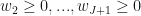
ggplot(plot.df,aes(x=year,y=y,color=unit)) + geom_line() + ylab("") + scale_color_manual(values=c('black','red')) +
ggtitle('GDP per capita among rural counties') +
theme_tufte()
####################################################################
####################################################################
####################################################################
####################################################################
Some Final Thoughs
Like most things I write about, I don’t think one can really do the topic justice in a single post. Here are a few things I didn’t really touch on:
1. Synthetic Control is about more than just drawing a line for a treated unit and comparing that line with a line drawn for the synthetic unit (representing the credible counterfactual). Dealing with statistical inference and uncertainty in comparative case studies is tricky for a variety of reasons. The Synthetic Control methodology has some features that lends themselves pretty nicely to conducting statistical inference and quantifying the uncertainty associated with estimates.
2. Using the Synthetic Control model, one can derive both the traditional Difference-in-Differences estimator and the Dynamic Factor Model.
Hopefully, at some point in the not too distant future, I’ll get around to writing a second post on placebo-type techniques for generating confidence intervals around Synthetic Control estimates.

Hi, thanks for your interesting post. I tried to reproduce your example however struggle somehow to understand where the object synth.data come from, at least its not in the global environment.
Appreciate your comment.
Thanks Alex
Hi Alex,
Once I’ve loaded the ‘Synth’ package into the workspace I’m able to load the data synth.data successfully using: data(synth.data). My example works with data that is slightly altered from the ‘synth.data’ that ships with the Synth package (it’s pretty close but I’ve found my students respond a bit more enthusiastically to natural resource related examples so I’ve changed a few names and things like that). If you are trying to follow along with my example I suggest copying the data from the text in the blog post. My code here uses ‘fracking.data’ not ‘synth.data’…or at least I think it does. If you’re still having trouble perhaps you can identify which code chunk and line from the post references ‘synth.data’ that you’re having trouble with.