
Natural resource economists such as myself spend a fair amount of time obsessing over how things are distributed in space. This is because we spend a lot of time dealing with environmental data that tend to have important spatial characteristics:
- water quality observations taken at two nearby monitoring stations may produce similar values as chemical concentrations in groundwater aquifers may be localized.
- mineral concentrations at two nearby testing locations will tend to be similar due to basic geological characteristics
- fishing success may be spatially correlated if fish tend to concentrate in certain areas due to habitat preferences
I’m going to break this post up into 2 things I enjoyed doing this week. The first was really basic: plotting some point data with lat/long coordinates on top of static google maps using gg_map, ggplot and a few other R packages for geospatial type stuff. The second was a little more involved but still accessible enough for a blog: using the SPDEP package to run some spatial statistics.
Really Basic Mapping
The setting for this exercise is the following: I’m working with a graduate student who is interested in the potential impacts of hydraulic fracturing in California on i) surface water quality in general, ii) groundwater quality in general, and iii) water quality in watersheds supporting threatened and endangered species (like coho salmon and steelhead). In California there are two main shale formations that are being mined (via fracking and horizontal drilling) for oil: the Monterey and Santos Shale Formations. The Santos Shale runs under some ecologically important fish habitat in San Luis Obispo, Santa Barbara, and Ventura Counties. These areas have several small coastal streams and a few bigger rivers (like the Ventura and Santa Ynez) that support dwindling populations of protected species like Steelhead. As a result there is a non-trivial amount of hydraulic fracturing going on quite close to some pretty sensitive watersheds.
The student I’m working with has collected a ton of data on i) water quality at thousands of monitoring stations in CA, ii) oil production from hydraulically fractured wells in CA, and iii) disposal of fracking wastewater through injection into deep aquifers.
One of the first things I like to do when working with a new spatially explicit data set is visualize the spatial distribution of important variables. There are several ways to do this in R but I really like the ggmap package that can be used with ggplot to plot points on top of a static google map.
There are some really nice walk-throughs online here, here, and here…
I’m going to start with a really basic map of where some of the hydraulically fractured wells in the data are located. Here is a snippet of my data in case you want to try this out (for the actual analysis this location info in linked to a few other tables that have monthly production levels for each well and water quality observations for each monitoring station within a few different specified distance bands of each well…but for now I’m just interested in putting these on a map to see where they are).
Here is the data I have saved in an object called vwells:
APINumber| OperatorName| Latitude| Longitude| SPUDDate
280434 11122182| Vintage Production California LLC| 34.36465| -118.9195|
284389 11100000| Union Oil Company of California| 34.41146| -119.1120|
284390 11100001| Aera Energy LLC| 34.32134| -119.2468| 12/21/47
284391 11100002| PRE Resources, LLC| 34.41506| -118.9101| 6/11/59
284392 11100003| Chevron U.S.A. Inc.| 34.41780| -118.9069| 9/30/59
284393 11100004| Chevron U.S.A. Inc.| 34.41479| -118.9098| 2/19/60
284394 11100005| Fillmore Land Co.| 34.42032| -118.9004| 8/21/60
284395 11100006| Chevron U.S.A. Inc.| 34.41642| -118.9136| 12/24/60
284396 11100007| Chevron U.S.A. Inc.| 34.42299| -118.9065| 6/22/61
284397 11100008| Chevron U.S.A. Inc.| 34.41768| -118.9175| 6/22/61
284398 11100009| Santa Fe Minerals, Inc.| 34.40318| -118.9335|
284399 11100010| Santa Fe Minerals, Inc.| 34.40453| -118.9359|
284400 11100011| Chevron U.S.A. Inc.| 34.40160| -118.9361| 9/14/57
284401 11100012| Chevron U.S.A. Inc.| 34.41410| -118.9136|
284402 11100013| Chevron U.S.A. Inc.| 34.41419| -118.9137|
284403 11100014| Chevron U.S.A. Inc.| 34.40405| -118.9245|
284404 11100015| Chevron U.S.A. Inc.| 34.40883| -118.9221|
284405 11100016| Chevron U.S.A. Inc.| 34.40374| -118.9445|
284406 11100017| Chevron U.S.A. Inc.| 34.40561| -118.9409|
284407 11100018| Chevron U.S.A. Inc.| 34.40477| -118.9473|
require(ggmap)
require(maps)
require(ggplot2)

map <- get_map(location="Santa Paula",zoom=10,maptype="terrain")
ggmap(map) +
  geom_point(aes(x=Longitude,y=Latitude),size=5,
             shape=17,data=vwells)
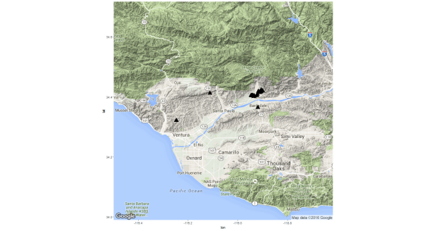
From the map we can see a somewhat disturbing fact: there appears to be a pretty big cluster of fracking activity right along the Ventura River and some activity not far from Santa Paula Creek. This isn’t really bad per se but it is somewhat worrisome that, in an area that has already experienced massive degradation to aquatic habitat and where a considerable amount of money is being spent to recover an ESA-listed species (steelhead trout), we have what looks to be a decent amount of oil production going on via hydraulic fracturing (a practice which is known to have both i) persistent small environmental impacts (consistent leakages of fracking fluid into groundwater and surface water supplies) and ii) risks of potentially catastrophic events.
Maybe I’ll talk more about this project another time, for the moment let’s move on the some spatial stats.
Spatial Autocorrelation with Moran’s I and Ape
Another data set I’m working with at the moment pertains to catches in a commercial capture fishery. My research group is particularly interested in how changes in the spatial distribution of fish species resulting from a changing climate may impact coastal communities where commercial fishing is an important driver of local economic conditions. An important foundation for this research is a basic understanding of how spatially correlated commercial fishing outcomes are.
Unfortunately I cannot share these data because they are not mine to share. For the remainder of this discussion let’s assume we have a data frame called df.tmp with the following characteristics:
vessel_id| trip_id| haul_id| gear| set_lat| set_depth| set_long| lbs|date|depart_port| species
1| 1| 1| bottom trawl|36.721|-124.56|210|175|2011-01-01|PortName1| fish1
1| 1| 1| bottom trawl|36.721|-124.56|210|110|2001-01-01|PortName1| fish2
1| 1| 2| bottom trawl|36.69|-124.6|220|250|2011-01-01|Portname1|fish1
This is probably a good time to slow down and explain some terminology: My data pertains to vessels that take fishing trips lasting anywhere from 1 – 5 days. On each trip the vessel may initiate several hauls. A haul refers to one set of the fishing gear (if the vessel is using trawl gear then this is one ‘drag’ of the trawl net….if the vessel is using hook-and-line gear, a haul would be one set of the hook-and-line gear). Each haul may bring in several different species. The data are organized such that each species landed on each haul gets its own row.
Moran’s I is a measure of how correlated a signal is at across space. It is sometimes used as index of clustering as it basically assesses whether values at nearby locations tend to be more or less similar than values at locations that are far apart.
For the rest of this post I’m going to walk through an example of calculating the Moran’s I statistic (a good primer is contained in the slides here: http://www-hsc.usc.edu/~mereditf/Spatial%20Statistics%206.pdf) at two different resolutions.
The first pass here is to calculate the Moran’s I statistic to get a feel for how spatially correlated fishing outcomes are. I did this first using each haul in the data set.
So an important thing to note when we calculate Moran’s I using all the hauls in the data is that this might mix a spatial effect with an individual effect. In my opinion there is kind of an interesting duality here:
- On one hand, if you are a biologist concerned with making inference on how many fish are in some part of the ocean based on how many fish a vessel is able to catch in that area in a given time period, you might want lots of observations by the same vessel (ideally a research vessel where the parameters of fishing activity are know and hopefully were designed in such a way as to provide accurate, valuable information). This is because if you observe many hauls by the same vessel in an area you are effectively holding constant all the individual-specific factors that might influence fishing success…meaning that any variation you observe in catch from one location to another is likely due to the density of fish in those locations and not due to different fishing tactics or practices.
- On the other hand, if you’re an economists, you might be more interested in whether fishing success tends to be correlated when measured at two nearby locations but for different vessels. Do fishermen sharing similar fishing grounds tends to experience similar outcomes?
The Moran’s I statistic is defined as:

In this specific case 


From the formula one can see that that weight attached to the relationship between observation
- Binary weights. Using this type of weighting,
- Continuous weights where the elements
To use the function Moran.I from the R package ape we supply a vector of values (x) that we want to test for spatial autocorrelation (in our case the lbs of fish landed on each fishing event) and a weights matrix that defines how row
For this application I’m going to define the weights (
#great circle distance between two sets of lat/long
dist.fn <- function(p1,p2){
#input should be entered such that p1=(latitude 1, longitude 1) and p2=(latitude 2, longitude 2)

#convert to radians
  p1 <- (p1*pi)/180
  p2 <- (p2*pi)/180

  a <- sin((p2[1]-p1[1])*0.5)*sin((p2[1]-p1[1])*0.5) +
    sin((p2[2]-p1[2])*0.5)*sin((p2[2]-p1[2])*0.5)*cos(p1[1])*cos(p2[1])
  c <- 2*atan2(sqrt(a),sqrt(1-a))
#normalize by approximate circumference of the earth
 d <- c*6371
return(d)
}
The next step is to define the weighting matrix that will be feed into the function Moran.I…but first I do a few dplyr gymnastics because I want to use certain subsets of the data. Basically, I only want to compare fishing events if they occurred in the same season (there are biological and physical reasons to believe fishing success at a particular location will vary seasonally), and in the same general depth zone (the continental shelf and continental slope are very different environments and it is a generally accepted biological fact that two fishing events could be quite close together as measured along an east-west distance and have very different outcomes by virtue of being at different depths and therefore fishing in distinct marine environments…I’m going to control for this by only comparing fishing events that happen in the same biogeographic zones.)
require(dplyr)
require(lubridate)

sar.df <- df.tmp %>% filter(depart_port %in% c('EUREKA','FORT BRAGG','SAN             FRANCISCO','SAN FRANCISCO AREA',
'BODEGA BAY','PRINCETON (HALF MOON BAY)','MONTEREY',
'MOSS LANDING','MORRO BAY','AVILA')) %>%
 mutate(zone=ifelse(set_depth<=75,1,ifelse(set_depth>=100,2,0))) %>% #set a variable for seaward or shoreward of the RCA
   group_by(vessel_id,trip_id,haul_id,gear,date) %>%
summarise(lbs=sum(lbs),lat=unique(set_lat),
          long=unique(set_long),dport=unique(departure_port),
month=unique(month(date)),
year=unique(year(date)),
zone=max(zone)) %>%
   mutate(season=ifelse(month(date) %in% c(1,2,3),'winter',
          ifelse(month(date) %in% c(4,5,6),'spring',
          ifelse(month(date) %in% c(7,8,9),'summer','winter'))))
Ok, so with that out of the way we can set up the spatial weights matrix. The way I’m going to set up weights here is to use the physical distance between two fishing events.
I’m also going to wrap the distance calculations and the call to the Moran.I function in a function of my own because I want to be able to investigate different spatial scales…that is, I want to be able to calculate the statistic using only observations from the same port (a local measure of clustering) and then, more globally, using all observations from several ports. The following function does three basic things:
- filters the data to meet user defined criteria
- computes a spatial weights matrix (
- invokes the function Moran.I from the ape package to estimate Moran’s I for the data
#a function to get the Moran's I statistic for data points meeting certain criteria
moran.fn <- function(port.now,gear.now,month.now,year.now,zone.now){

#here we set up the data that will feed into the Moran.I function
    data <- sar.df %>% filter(dport %in% port.now & month %in% month.now & year %in% year.now & lbs>0 & gear %in% gear.now & zone %in% zone.now)

#set up an N X N matrix that will be populated such that the entry in
# row i and column j will be the distance between observation i and j
  sar.dist <- matrix(0,nr=nrow(data),nc=nrow(data))

#populate the distance matrix using repetitive calls to the distance function
# we wrote earlier
  for(i in 1:nrow(sar.dist)){
    loc1 <- c(sar.dist$lat[i],sar.dist$long[i])
    for(j in 1:nrow(sar.dist)){
      loc2 <- c(sar.dist$lat[j],sar.dist$long[j])
      d <- dist.fn(p1=loc1,p2=loc2)
      sar.dist[i,j] <- d
    }
  }

#transform the distance calculation to be the inverse distance
  sar.dist <- 1/sar.dist
  diag(sar.dist) <- 0
#get rid of any infinite values in the matrix
  sar.dist[is.infinite(sar.dist)==T] <- 0
#call the function Moran.I and return the results
  return(list(nobs=nrow(data),Moran.I(data$lbs,sar.dist)))

}
So now I’ll call this function and declare that I want to include all fishing events off the Coast of California in my calculation, but I only want observations from the same year, same season, and for fishing events that utilize the same type of fishing gear.
#Moran's I using all summer 2011 obs coastwide...bottom trawl gear only
 moran.fn(port.now=c('EUREKA','FORT BRAGG','PRINCETON (HALF MOON BAY)',
             'BODEGA BAY','SAN FRANCISCO','SAN FRANCISCO AREA','MORRO BAY','AVILA',
             'MONTEREY','MOSS LANDING'),gear.now='Bottom Trawl',month.now=c(7,8,9),
          year.now=2011)
$nobs
[1] 1045

[[2]]
[[2]]$observed
[1] 0.3250107

[[2]]$expected
[1] -0.0009578544

[[2]]$sd
[1] 0.007764127

[[2]]$p.value
[1] 0
Here, the positive value with significant p-value indicates positive and significant spatial autocorrelation.
Moran’s I is a measure of how similar two things are that are close together. In these data, 2 hauls are likely to be relatively close together if they were performed by the same fisherman on the same fishing trip. So if Moran’s I confirms that the fishing outcomes are spatially correlated, it may be because fish tend to cluster in preferred habitats, and it may also be because the two hauls were performed by the same fisherman.
With that in mind, next, I want to evaluate Moran’s I using only data for which each observation represents a different fisherman. I’m going to do that using the following approach:
- assign each fishing trip to a location by calculating the midpoint of all fishing events on the same fishing trip
- randomly sample one trip for each fisherman in the data sample
- use Moran’s I to assess spatial autocorrelation in landings at the trip level.
#Next, we want to try to represent each fishing trip by it's locational center and compare
# spatial correlation in landings for fishing trips....this is to address any possible bias
# introduced by just comparing the first tow of each vessel

moran.trips <- df.tmp %>% filter(d_port %in% c('EUREKA','FORT BRAGG','SAN FRANCISCO','SAN FRANCISCO AREA',
                                          'BODEGA BAY','PRINCETON (HALF MOON BAY)','MONTEREY','MOSS LANDING','MORRO BAY','AVILA')) %>%
  mutate(zone=ifelse(set_depth<=75,1,ifelse(set_depth>=100,2,0))) %>% #set a variable for seaward or shoreward of the RCA
  group_by(drvid,trip_id,haul_num,sector,geartype) %>%
  summarise(lbs=sum(ret),lat=unique(set_lat),long=unique(set_long),port=unique(d_port),month=unique(set_month),year=unique(set_year),
            zone=max(zone))

moran.locs <- moran.trips %>% mutate(x=cos(lat*(pi/180))*cos(long*(pi/180)),
                                     y=cos(lat*(pi/180))*sin(long*(pi/180)),
                                     z=sin(lat*(pi/180))) %>% #convert lat/long to radians then cartesian coordinates
                group_by(trip_id) %>%
                summarise(mean.x=mean(x),mean.y=mean(y),mean.z=mean(z)) %>%  #get average coordinates
                mutate(long.center=atan2(mean.y,mean.x),
                       hyp=sqrt((mean.x*mean.x)+(mean.y*mean.y)),
                       lat.center=atan2(mean.z,hyp)) %>% #convert back to lat/long radians
                mutate(lon.c=long.center*(180/pi),
                       lat.c=lat.center*(180/pi)) %>% #convert back to decimal degrees
                select(trip_id,lat.c,lon.c)

#merge the trip midpoint info with the original info
moran.trips <- moran.trips %>% inner_join(moran.locs,by='trip_id') %>%
              group_by(trip_id) %>%
              mutate(n_gear=n_distinct(geartype)) %>%
              filter(n_gear==1) %>%
              group_by(sector,drvid,trip_id,month,year,port) %>%
              summarise(lbs=sum(lbs),gear=unique(geartype),
                        zone=max(zone),lat=max(lat.c),long=max(lon.c))
Now I use the same function to get Moran’s I that I used earlier with one little tweak: I use the sample_n() function in dplyr to select a random fishing trip for each vessel (this way there is only 1 observation per vessel in the final data I use in the calculation of Moran’s I).
moran.fn <- function(port.now,gear.now,month.now,year.now,zone){
data <- moran.trips %>% filter(port %in% port.now & month %in% month.now &
year %in% year.now & lbs>0 & gear %in% gear.now) %>%
group_by(drvid) %>%
sample_n(1)
sar.dist <- matrix(0,nr=nrow(data),nc=nrow(data))
for(i in 1:nrow(sar.dist)){
loc1 <- c(data$lat[i],data$long[i])
for(j in 1:nrow(sar.dist)){
loc2 <- c(data$lat[j],data$long[j])
d <- dist.fn(p1=loc1,p2=loc2)
sar.dist[i,j] <- d
}
}
sar.dist <- 1/sar.dist
diag(sar.dist) <- 0
sar.dist[is.infinite(sar.dist)==T] <- 0
return(list(nobs=nrow(data),Moran.I(data$lbs,sar.dist)))
}
Call the function the same way we did for the case where we included all observations:
moran.fn(port.now=unique(moran.trips$port),gear.now='Bottom Trawl',month.now=c(7,8,9),year.now=2012,zone=2)
$nobs
[1] 20

[[2]]
[[2]]$observed
[1] 0.2506691

[[2]]$expected
[1] -0.05263158

[[2]]$sd
[1] 0.1296109

[[2]]$p.value
[1] 0.01927931
Here, results indicate that trips located closer together tend to land similar amounts of fish (the Moran’s I statistic is positive at 0.251 and significant with a p-value of approximately 0.02)
There are a lot of other techniques (both statistical and graphical) that we might want to use to characterize the spatial properties of our data…I’ll try to address some of those in the future.
