
In a previous post I illustrated a few really cool features of the Quantmod package in R. More specifically, I have been using Quantmod to pull historical pricing data on stocks and mutual funds directly from Yahoo Finance into R.
I’ve streamlined a few things from that post which I will show you here. I still don’t have a full-scale portfolio analyzer ready to unveil but I’ve made a few code tweaks that some of you might find useful.
First I should say: the Quantmod package has a lot of cool features built in for charting financial data and doing technical analysis (Bollinger Bands, MACD, etc., etc.). However, I’ve had a little trouble dealing with multiple different assets in the Quantmod environment. This might be because I have a lot of time invested in the dplyr way of dealing with data frames and I’m not as familiar with xts objects. So one of my big challenges has been how to efficiently build a dplyr data frame with asset price data pulled from Yahoo Finance.
Here I’m going to do something really simple: use the mutual fund screener in Fidelity to identify some of the top performing small and mid-cap growth funds, then use Quantmod to pull historical data for those funds, and finally, I’m going to plot the growth of a hypothetical $10,000 invested in each of the funds over different time horizons.
require(Quantmod)
require(data.table)
require(dplyr)

df.pull <- function(tickers,startDate,endDate){
stockData <- new.env() #Make a new environment for quantmod to store data in

#Download the stock history (for all tickers)
getSymbols(tickers, env = stockData, src = "yahoo", from = startDate, to = endDate)

#first coerce the environment to a data frame....this gives us a list of
# data frames
df2 <- eapply(stockData,as.data.frame)

#now if we change the column names in each of the list objects we can use
# rbindlist to get them in a single data frame...the problem  here is that
# the assets are not in the data frame 'df2' in the same order I put them in
# the object 'tickers'.  For each data frame in the list I need to recover the name
# of the asset and also give the columns new names.
df.clean <- function(tmp.data){
  asset <- unlist(strsplit(names(tmp.data)[1],"[.]"))[1]
  names(tmp.data) <- c("Open","High","Low","Close","Volume","Adjusted")
  tmp.data$asset<-asset
  tmp.data$date <- as.Date(row.names(tmp.data),format="%Y-%m-%d")
  return(tmp.data)
}
#apply the function above to each element in the df2 list...then coerce the output
# to a data frame
return(tbl_df(data.frame(rbindlist(lapply(df2,df.clean)))))
}
The function above accepts as inputs:
- a character vector of ticker symbols for the assets I want historical prices for
- a starting date and ending date which should both be date class object
And returns a dplyr data frame with daily prices for each of the assets passed into the function.
So now I’m going to use my data pull function to get some historical data on mutual funds that I identified using Fidelity’s Fund screener – I basically used the screener to look for funds with a high Morningstar rating, low expenses, above average returns, and funds of the class ‘small-cap growth’ or ‘mid-cap growth.’ The assets I chose for this are:
- BUFTX – Buffalo Discovery Fund
- FCPGX – Fidelity Small Cap Growth Fund
- FDEGX – Fidelity Growth Strategies Fund
- IWB – This is the exchange traded fund for the Russell 1000 Small Cap index…I included this as a benchmark
- FMCSX – Fidelity Mid Cap Stock Fund
- VISGX – Vanguard Small Cap Growth Index
- VMGRX – Vanguard Mid Cap Growth Investor Class
- I’m going to feed these ticker symbols into my function, get the daily prices, and then roll the daily data up to a monthly data frame:
#declare what ticker symbols I want
tickers <- c('BUFTX','FCPGX','FDEGX','IWB','FMCSX','VISGX','VMGRX')

#pull the data
funds <- df.pull(tickers=tickers,startDate=as.Date('1995-01-01'),
                 endDate=as.Date('2016-01-01'))

#aggregate the data to monthly values
funds.m <- funds %>% mutate(year=year(date),month=month(date)) %>%
  group_by(asset,month,year) %>%
  summarise(Low=min(Low),High=max(High),Close=last(Adjusted)) %>%
  group_by(asset) %>% arrange(asset,year,month) %>%
  mutate(MA3=rollmean(x=Close,3,align='right',fill=NA),
         MA6=rollmean(x=Close,6,align='right',fill=NA),
         MA9=rollmean(x=Close,9,align='right',fill=NA),
         growth=(Close-lag(Close))/lag(Close),
         date=as.Date(paste(year,"-",month,"-",'01',sep=""),format="%Y-%m-%d"))
Next, I’m going to write a pretty simple function to calculate the growth of a hypothetical $10,000 invested in each asset. I’m once again going to allow start date and end date to be inputs to the function so I can look at how these assets have performed over different past time periods.
growth.fn <- function(startdate,enddate,asset.names){
  tmp <- funds.m %>% filter(date>=startdate & date<=enddate & asset %in% asset.names)
  r <- lapply(unique(tmp$asset),function(a){
    val<-list()
    k<-0
    for(i in 1:length(tmp$date[which(tmp$asset==a)])){
      d<-tmp$date[which(tmp$asset==a)][i]
      if(i==1){
        v=10000
      }else{
        v=v*(1+tmp$growth[which(tmp$asset==a & tmp$date==d)])
      }
      val[[i]]<-v
    }
    return(data.frame(asset=a,date=tmp$date[which(tmp$asset==a)],val=unlist(val)))
  })

r <- data.frame(rbindlist(r))
tmp <- tmp %>% inner_join(r,by=c('asset','date'))
return(tmp)
}
Note that I can control the assets to be analyzed using the asset.names argument but – and this may be a little pedantic – the function works with the data stored in the object funds.m so I can only feed it asset names that exist in the funds.m data frame.
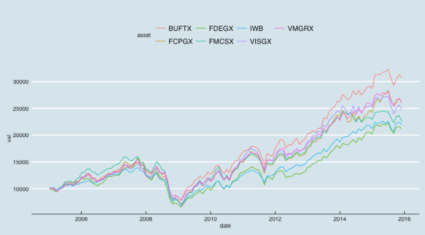
#declare assets
tickers <- c('BUFTX','FCPGX','FDEGX','IWB','FMCSX','VISGX','VMGRX')
#establish start date
startdate <- '2005-01-01'
#establish end date
enddate <- '2015-12-01'
#declare which assets in 'ticker' I want to include in the comparison
asset.names <- tickers

#call the growth function and plot results
z<-growth.fn(startdate=startdate,enddate,asset.names=unique(funds.m$asset)) ggplot(z,aes(x=date,y=val,color=asset)) + geom_line() #print the final value for each asset z %>% filter(date==enddate) %>% select(asset,date,Low,High,Close,val) %>%
  ungroup() %>% arrange(-val)

  asset       date    Low   High  Close      val
  (chr)     (date)  (dbl)  (dbl)  (dbl)    (dbl)
1 BUFTX 2015-12-01  19.30  21.65  19.62 30761.49
2 VMGRX 2015-12-01  21.98  25.22  22.45 26075.07
3 FCPGX 2015-12-01  18.50  19.49  18.70 26039.90
4 VISGX 2015-12-01  33.56  35.72  34.18 24785.93
5 FMCSX 2015-12-01  32.11  36.35  32.73 22556.89
6   IWB 2015-12-01 111.04 117.45 113.31 21984.91
7 FDEGX 2015-12-01  32.76  34.31  33.28 21212.71
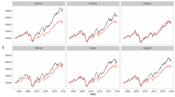
And if we want to visualize how each individual fund performs relative to the IWB small cap index we could use ggplot, facet on the asset name and add a common reference line like this:
iwb <- z[z$asset=='IWB',]
ggplot(subset(z,asset!='IWB'),aes(x=date,y=val)) + geom_line() +
  facet_wrap(~asset) +
  annotate(geom='line',x=iwb$date,y=iwb$val,color='red')  +
  theme_bw()
I have a few more little tweaks to share but I’ll start a new post for those.
